Now, that we've learnt how to enter dates and time to your spreadsheet, it's time to talk about the ways of calculating time in Google Sheets. We'll discuss the ways of finding time difference in detail, see how to sum dates and time together, and learn to display only date or time units and set them apart completely.
How to calculate time difference in Google Sheets
When you're working on some projects, it is usually important to control how much time you spend. This is called elapsed time. Google Sheets can help you calculate the time difference in a lot of various ways.
Example 1. Subtract time to get the time duration in Google Sheets
If you have your start time and end time, it's not a problem to find out the time spent:
Let's assume the start time is in column A and the end time is in column B. With a simple subtraction formula in C2, you will find how much time this or that task took:
=B2-A2
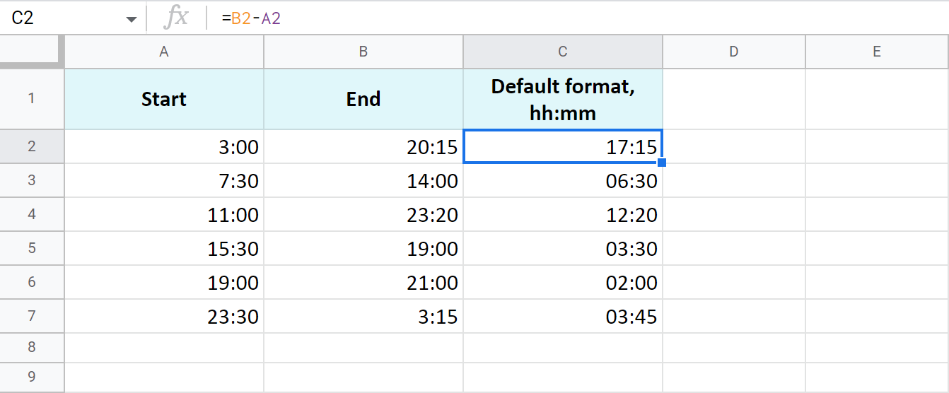
The time is formatted as "hh:mm" by default.
To get the results as hours only or as hours, minutes, and seconds, you need to apply a custom format with the corresponding time codes: h and hh:mm:ss. Google even offers a special number format for cases like this - Duration:
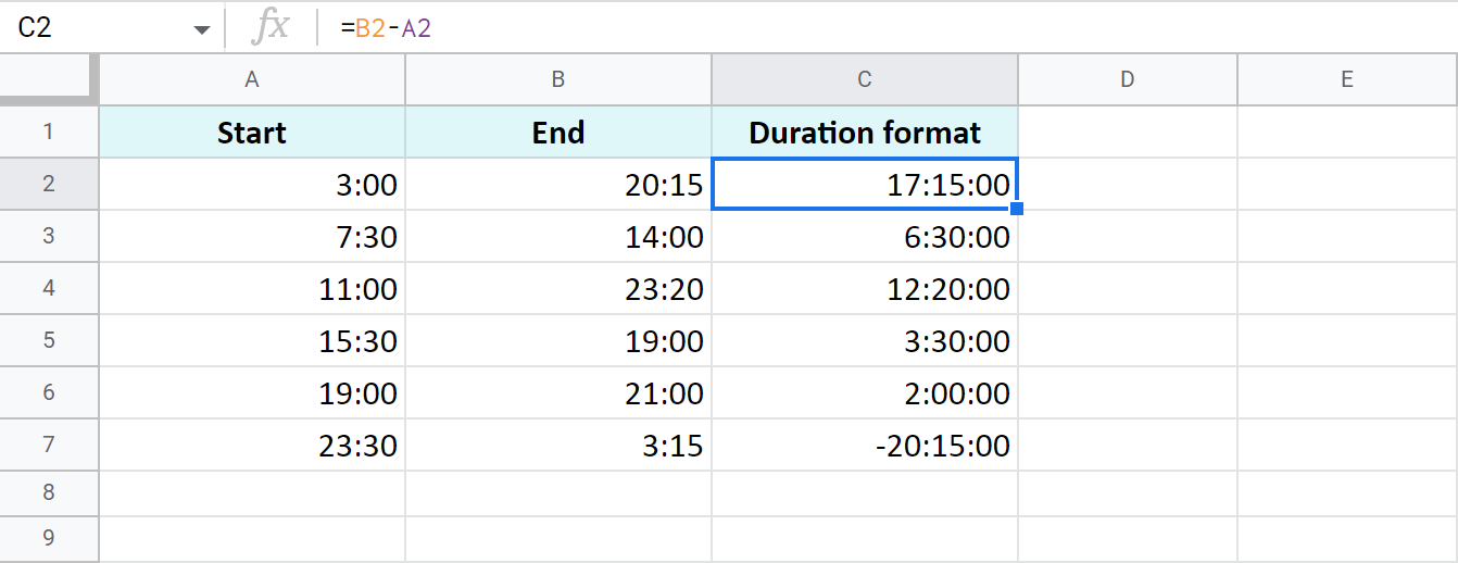
Tip. To apply the custom time format, go to Format > Number > Custom number format in your spreadsheet menu.
Example 2. Calculate time duration in Google Sheets using the TEXT function
Another trick to calculate the time duration in Google Sheets involves the TEXT function:
=TEXT(B2-A2,"h") - for hours
=TEXT(B2-A2,"h:mm") - for hours and minutes
=TEXT(B2-A2,"h:mm:ss") - for hours, minutes, and seconds
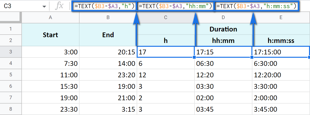
Note. See how the records are aligned to the left? Because the TEXT function always returns the results formatted as a text. This means these values cannot be used for further calculations.
Example 3. Time difference in hours, minutes, and seconds
You can track the time spent and get the result in one time unit disregarding other units. For example, count the number of only hours, only minutes, or only seconds.
Note. To ensure correct results, your cells should be formatted either as numbers or automatically: Format > Number > Number or Format > Number > Automatic.
-
To get the number of hours spent, subtract your start time from the end time and multiply the result by 24 (since there are 24 hours in one day):
=(End time - Start time) * 24You will get a time difference as a decimal:

If the start time is greater than the end time, the formula will return a negative number, like in C5 in my example.
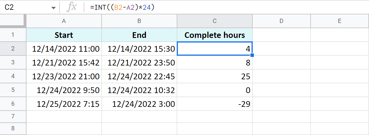
Tip. The INT function will let you see the number of complete hours spent since it rounds numbers down to the nearest integer:
-
To count minutes, subtract the start time from the end time and multiply whatever you get by 1,440 (since there are 1,440 minutes in one day):
=(End time - Start time) * 1440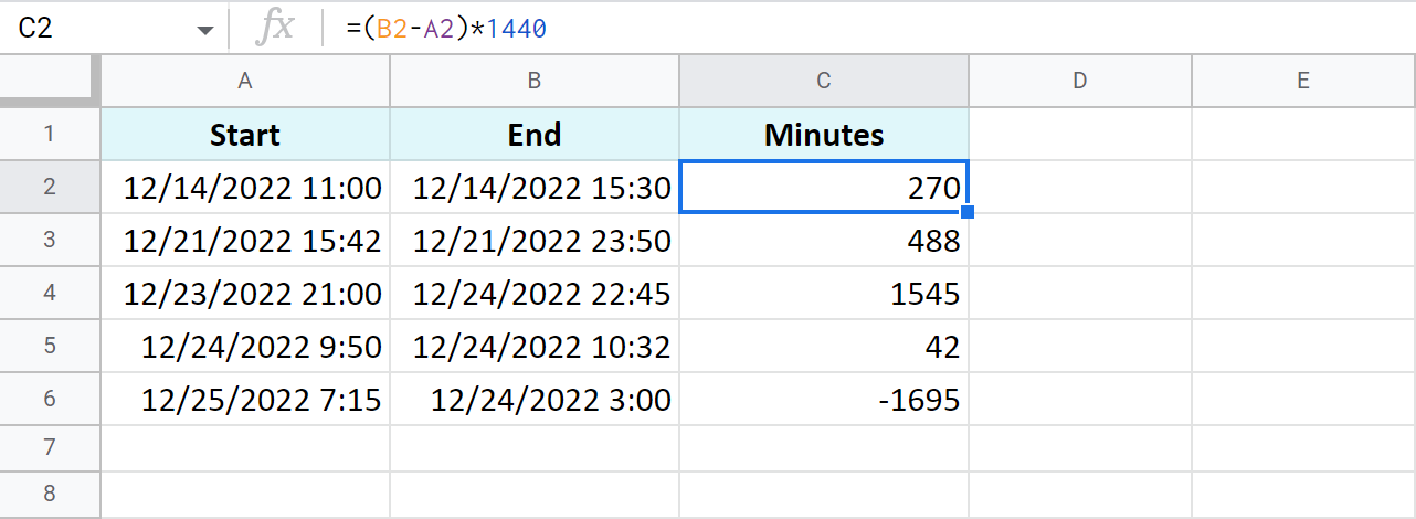
-
To find out how many seconds passed between two times, the drill is the same: subtract the start time from the end time and multiply the result by 86,400 (the number of seconds in a day):
=(End time - Start time) * 86400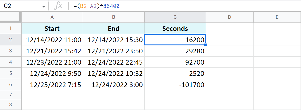
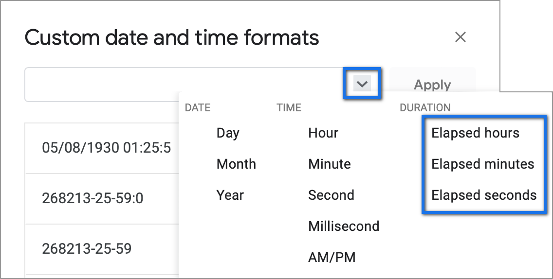
Tip. You can avoid multiplying in all these cases. Just subtract times first, and then apply elapsed time format from Format > Number > Custom date and time. If you click the down arrow to the right of the text field, you'll be able to choose between additional date and time units:
Example 4. Functions to get the time difference in a Google spreadsheet
As always, Google Sheets equips you with three particularly useful functions for this purpose.
Note. These functions work only within 24 hours and 60 minutes and seconds. If the time difference exceeds these limits, the formulas will return errors.
=HOUR(B2-A2)- to return hours only (without minutes and seconds)=MINUTE(B2-A2)- to return minutes only (without hours and seconds)=SECOND(B2-A2)- to return seconds only (without hours and minutes)

How to add and subtract time in Google Sheets: hours, minutes, or seconds
These operations can also be achieved with two techniques: one involves basic math calculations, another - functions. While the first way always works, the second one with functions works only when you add or subtract units less than 24 hours, or 60 minutes, or 60 seconds.
Add or subtract hours in Google Sheets
-
Add less than 24 hours:
=Start time + TIME(N hours, 0, 0)Here's how the formula looks on real data:
=A2+TIME(3,0,0)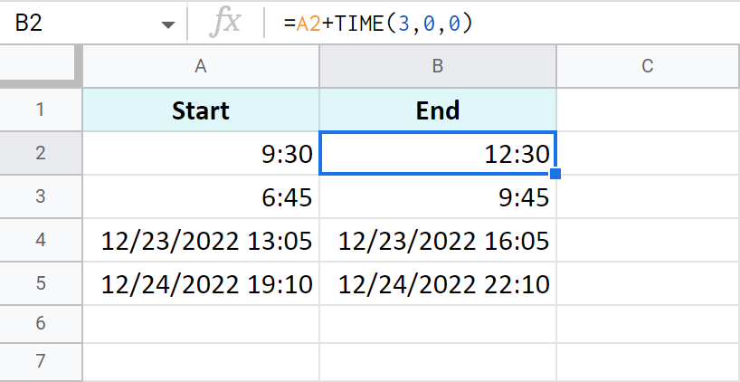
-
Add more than 24 hours:
=Start time + (N hours / 24)To add 27 hours to the time in A2, I use this formula:
=A2+(27/24)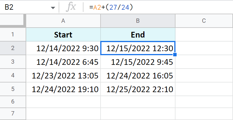
- To subtract 24 and more hours, use the formulas above as a basis but change the plus sign (+) to the minus sign (-). Here's what I've got:
=A2-TIME(3,0,0)- to subtract 3 hours=A2-(27/24)- to subtract 27 hours
Add or subtract minutes in Google Sheets
The principle of manipulating minutes is the same as with the hours.
-
There's the TIME function that adds and subtracts up to 60 minutes:
=Start time + TIME(0, N minutes, 0)If you are to add 40 minutes, you can do it like this:
=A2+TIME(0,40,0)If you are to subtract 20 minutes, here's the formula to use:
=A2-TIME(0,40,0)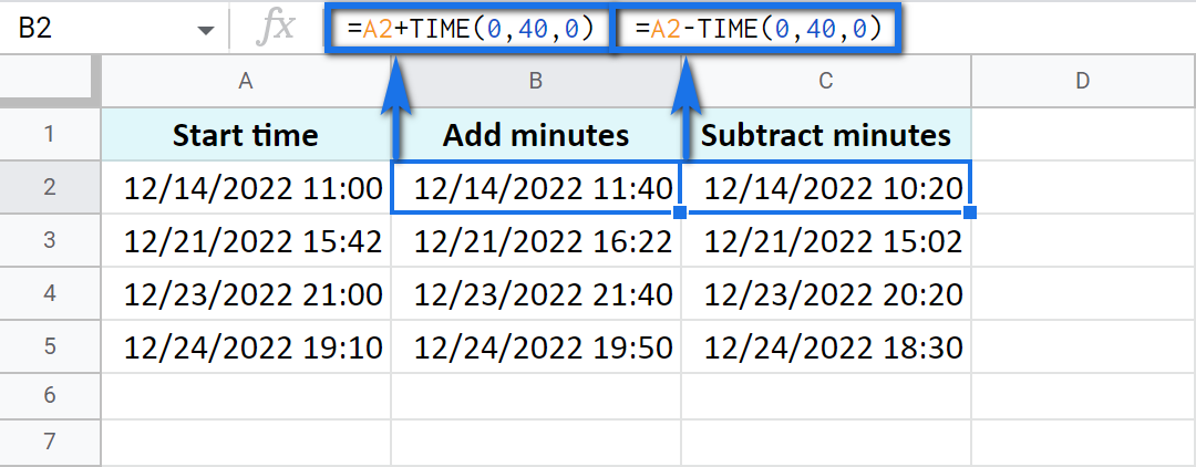
-
And there's a formula based on simple arithmetic to add and subtract over 60 minutes:
=Start time + (N minutes / 1440)Thus, here's how you add 120 minutes:
=A2+(120/1440)Put the minus instead of plus to subtract 120 minutes:
=A2-(120/1440)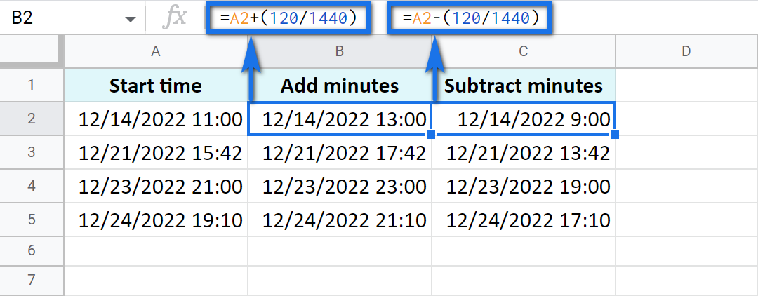
Add or subtract seconds in Google Sheets
Seconds in Google Sheets are calculated in the same manner as hours and minutes.
-
You can use the TIME function to add or subtract up to 60 seconds:
=Start time + TIME(0, 0, N seconds)For example, add 30 seconds:
=A2+TIME(0,0,30)Or subtract 30 seconds:
=A2-TIME(0,0,30) -
To calculate over 60 seconds, use simple maths:
=Start time + (N seconds / 86400)Add 700 seconds:
=A2+(700/86400)Or subtract 700 seconds:
=A2-(700/86400)
How to sum time in Google Sheets
To find the total time in your table in Google Sheets, you can use the SUM function. The trick here is to choose the correct format to display the result.
By default, the result will be formatted as Duration - hh:mm:ss
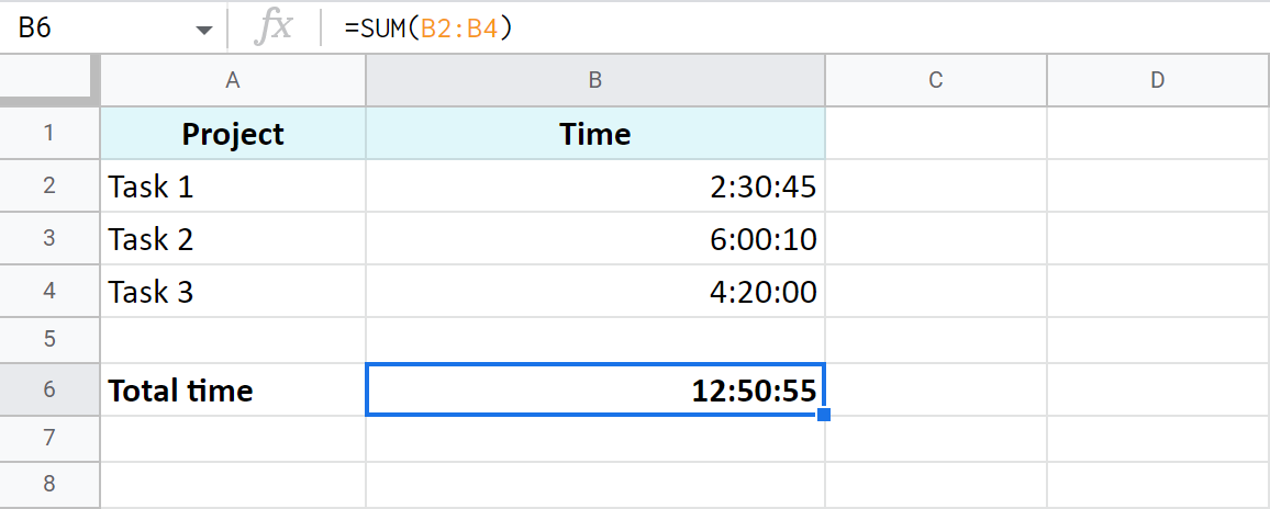
But most often the default time or duration format won't be enough, and you will need to come up with your own one.
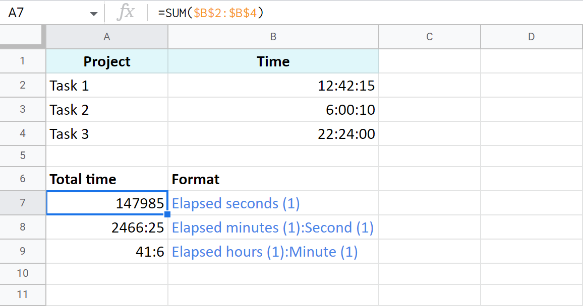
A7:A9 cells contain the same time value. They are just displayed differently. And you can actually perform calculations with them: subtract, sum, convert to decimal, etc.
Extract date and time from a full "date-time" record
Let's imagine that one cell in Google Sheets contains both, date and time. You want to set them apart: extract only the date to one cell and only time to another.
Split Date time using Number format
In order to display date or time in one cell on your screen or to print it, just select the original cell, go to Format > Number and choose Date or Time.
However, if you'd like to use these values for future calculations (subtract, sum, etc.), this won't be enough. If you don't see the time unit in a cell, it doesn't necessarily mean that it's absent, and vice versa.
So what do you do?
Split Date time using formulas
Google stores dates and time as numbers. For example, it sees the date 8/24/2017 11:40:03 as the number 42971,4861458. The integer part represents the date, the fractional - time. So, your task is down to separating integer from fractional.
- To extract date (integer part), use the ROUNDDOWN function in cell B2:
=ROUNDDOWN(A2,0)
The formula rounds the value down and casts the fractional part away.
-
To extract time, place the following subtraction formula into C2:
=A2-B2 -
Copy the results into the third row and apply Date format to B3 and Time format to C3:

Use the Split Date & Time add-on
You may be surprised but there's one special add-on for this job. It's really small and easy but its contribution to Google Sheets cannot be overstated.
Split Date & Time splits all Date time records in your entire column at once. You control the desired outcome with just 4 simple settings:
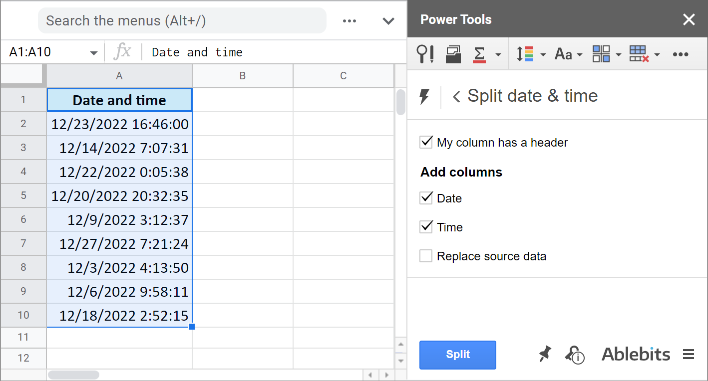
You tell the add-on:
- Whether there's a header row.
- If you want to get the Date unit.
- If you want to get the Time unit.
- And if you'd like to replace your original column with the new data.
It literally takes the burden of splitting date and time units off your shoulders:
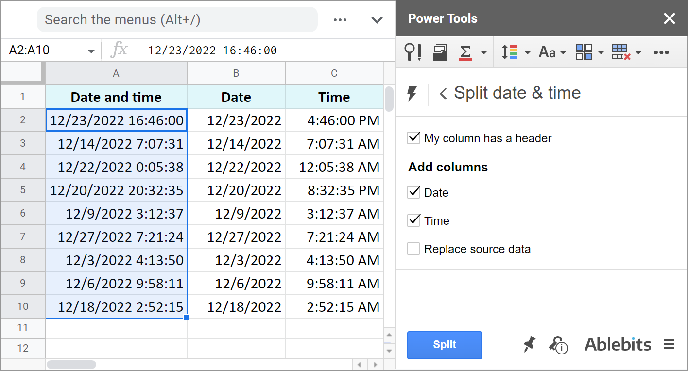
The add-on is part of the Power Tools collection so you will have more than 40 other useful add-ons at hand:
These are the ways to not only display date or time, but to separate them to different cells. And you can perform various calculations with these records now.
I hope these examples will help you solve your tasks when working with dates and time in Google Sheets.
Spreadsheet with formula examples
Calculating time in Google Sheets - formula examples (make yourself a copy)
 by
by 
372 comments
Hello, I am trying to add up all the time in one column and have it represented as dd:hh:mm but I just can't seem to do it. Im wondering if you could help. I will give an example directly from the sheet. Also, they are all represented as hh:mm. So c1, 0:41 c2, 0:53 c3, 2:22 c4, 3:28 c5, 9:17 c6, 6:49 c7, 1:56 c8, 3:25 c9, 2:43 c10, 6:28. Like asked how would I add the whole column with said outcome? (So if I update it time will change) Also, could these be averaged but with an outcome of hh:mm so I could find average hours per day? (Each c1, c2 ect is a day). Thank you so much this would be very appreciated.
Hello Jesse,
I answered the same question just a few days ago, please have a look :) The same formula will work for you. If you have your SUM in C11 (showing 38:02 as a result), reference C11 in the formula from that comment of mine, and you'll get 1 day 14 hours 2 minutes.
As for the average, it is usually calculated from a few values. I'm not sure how you want it to apply to each cell separately. Perhaps, you mean to round the values to full hours?
OH MY GOODNESS. Thank you this is awesome. ;)
Oh for the average just have it as it is hh:mm. I assume you naturally find the average then convert it with the formula you showed me. Hmmmm
Wait nevermind I figured out how to do the average.
It's my pleasure, Jesse :) Good to know you found the answer to your second question as well!
Sorry if this is a silly question. I want my time differences displayed as a decimal of an hour (1.5 hours instead of 1:30:00) How can I do this? Thanks!
Hello Moss,
I mention decimals in the following section: "Example 3. Time difference in hours, minutes, and seconds.". It's in the first part of the blog post, please take a look.
Also, here are some comments where I suggested formulas: SUM and convert to decimal, format values correctly to see decimals
Hi Natalia,
Firstly, thank you for the work you have done here, it has helped me a lot. However, I am stuck at the final hurdle.
I am calculating the total duration spent across a month and need to display the result in dd:hh:mm. I have the hh:mm for the month summed, so it's just this final part of the puzzle that has me stuck. Currently, I have a calculation that sums to 29:09 (so 29 hours and 9 minutes) which is correct and when I try to format that into dd:hh:mm it returns 31:05:09, however, it should be 01:05:09 (1 day, 5 hours and 9 minutes).
Hope you can help.
Thanks
John
Hi John,
Thank you for your feedback!
Please try the following formula instead (assuming your duration is in A2):
=INT(A2)&":"&IF(Hour(A2)<10,"0"&Hour(A2),Hour(A2))&":"&IF(Minute(A2)<10,"0"&Minute(A2),MINUTE(A2))
That's great! Thank you!
In regards to google sheets and changing the format. I imported a spreadsheet which has call log times for my employees. I am trying to standardize and find out the daily time they spend on the phones helping patients so I can track who is pulling the heaviest call volume. My report that exports from my phone company only puts the format as 10mins or 56 secs, is there a way or formula to convert that into the standard 00:00:00 timing format so that I can add up their total time? I am not seeing a way to do this and it is looking like this may be a manual process. Any help would be greatly appreciated.
Hello Mark,
There is a formula for your task :)
You can check if your cells contain 'mins' or 'secs' and extract the numbers already converted to minutes or seconds accordingly. Here's a formula:
=IF(ISNUMBER(SEARCH("mins",A2)),TIME(0,LEFT(A2,SEARCH("mins",A2)-1),0),IF(ISNUMBER(SEARCH("secs",A2)),TIME(0,0,LEFT(A2,SEARCH("secs",A2)-1)),""))
Paste this formula where you want to see the result, change A2 to a cell you're checking, and make sure to change the number format of the resulting cells to Duration.
Hy! I need to help to solve problem. When employee atrandece time is greater than office time than cell is colour red . How can it possible plz
Hi Muhammad,
You need to create a conditional formatting rule that compares data in two cells. We described how to do it in this blog post: Create Google Sheets conditional formatting based on another cell
I may be missing something, but I cannot find the solution to how to avoid a negative calculation of time when they're on two different days. I'm trying to create a very simple time sheet, but if someone has a start time of 11pm and end time of 4am this shows a total of -19 hours. How do we fix this within the formula? Thanks.
Hello Maria,
Please look at Example 1 in this part of the blog post. There's a similar case in row 3 and the subtraction works. Also, make sure you format your result cell correctly.
If you still can't get the required result, please tell me what you use as the start and end time exactly and specify your formula.
Thank you very much for the guide!
But I still experience an error that is testing my patient very hard...
Basically when i put 13:00 in a cell (after applying the hh:mm format) google sheet doesn't recognize that as a number or time and it says that it is text...
And no formulas works...
Only way that i found is to imput the time using . instead of : but it's a bad workaround
Anyone got this problem too?
Thanks!
Hi Manuel,
The date and time format and separators usually depend on your spreadsheet locale, time zone, and display language. I described it in this blog post, please have a look.
hello All, I have tried with formula, But giving the result as below, Please suggest what's wrong.
Eg : 05/06/2020 18:22:51 - 04/06/2020 16:42:24 = 721.6741667
Please suggest how to solve this
Thanks
Kantharaju
Hello Kantharaju,
Try selecting your resulting cell and changing its format to Duration.
I've two cells formatted as Date Time and i cannot do any calculation..
why? :(
Hello Mauro,
For me to be able to help you, please specify the formula that doesn't work and describe what lies in the ranges your formula refers to.
Hi,
This is a great website to learn excel from. I have a question, please reply me.
I have two columns, in one of the column there is duration and in the other one I want to add only the hours and not the minutes and seconds. For example: 1:45:30, 2:26:47 and 0:35:17 in column A, should appear as 1:00:00, 2:00:00 and 0:00:00 respectively in column B.
Is there any way
Hi Izhar,
Here's a formula for you to try if you work in Google Sheets:
=A2-MINUTE(A2)/1440-SECOND(A2)/86400
The basics of these are described in this paragraph above.
For formulas with time in Excel please visit this blog post: calculate time in Excel
what if i want to find the average of time with milliseconds, for example,
1:23.45
5:67.89
Hello David,
If the AVERAGE function returns errors, the problem is in the format of your source data. Google Sheets doesn't recognize the numbers you sent as numbers/time/duration. Also, the record 5:67.89 can't have 67 as seconds, the max can be 59.
So, please correct your records and go to the Format > Number to pick one of the existing formats. Or proceed to Format > Number > More Formats > More date and time formats to create a custom one.
Once it's correct, you'll be able to calculate the average even with milliseconds in time units.
I'm trying to count total days between 2 dates, but my time is first and then the date, example: (column k) 15:45 03/23/2020 and (column m) 00:01 3/25/2020.
Is this even possible? Thanks!
Hello Sarah,
Google Sheets will recognize and calculate your values only if they correspond to one of the existing formats (Format > Number in the menu). In this particular case, you should switch date and time units places. Such cells will then be formatted as Date time, and you'll be able to subtract one from another. (Otherwise, they are merely text strings and you won't be able to do anything with them.)
EXAMPLE #3 does not work correctly. I cannot get the elapsed time by hours in a decimal format with that formula.
Hello Emily,
Please specify your start and end time and check how these cells (including the one for the result) are formatted.
Also, please provide the exact formula you're using and whatever it returns to you.
I'll try my best to help.
Hi Natalia,
I have data with multiple times in a day formatted as start and stop times e.g.
1/1/2020 17:19 1/1/2020 19:22
1/1/2020 19:35 1/1/2020 20:25
1/1/2020 21:08 1/2/2020 1:21
1/2/2020 0:04 1/3/2020 17:30
1/2/2020 9:05 1/3/2020 6:30
I am trying to determine how much total time was used EXCLUDING overlaps. Can you suggest how this might be accomplished?
I figured this out by subtracting the previous end time from the next start time. Assuming the example I gave was 2 columns wide and 5 rows long this would be B1-A2.
Hi Tom,
My apologies I didn't manage to reply right away. Good to know you found an easy solution :)
=HOUR(SUM(E9-D9))+(MINUTE(SUM(E9-D9))/60)
Hi Kris,
This was the formula for Madden's case.
I'd advise you to omit the excess SUM parts. Also, if the start and end times are on different days (but the difference doesn't exceed 24 hours), you need to:
1) introduce the ABS function that turns the negatives into positives
2) subtract the time difference from 24 hours only when the difference is negative
Taking all these into account, here's the formula:
=IF((E9-D9)<0,24-HOUR(ABS(E9-D9))+(MINUTE(ABS(E9-D9))/60),HOUR(E9-D9)+(MINUTE(E9-D9)/60))
Hi natalia.
I tried your formula it worked but if the time starts for example at 5pm and ends in 1am it gets and error since it shows negative. What should be the right formula?
Hello,
I am using this template for a weekly timesheet: https://docs.google.com/spreadsheets/d/1qgfcWdcrxVSJu0HoyUZp7w4pGrtHoH7iu-nMe5Qb7To/edit#gid=874047713
I am trying to change the "Total Hours cells to show a decimal format rather an hour and minute format. I have tried adding the multiplication by 24 to the formula in the "Total Hours" cells and setting them to Automatic formatting, but rather than displaying as a decimal, they show an h:mm am/pm format. For example, when I applied it to a cell displaying a total of 1 and a 1/2 hours (1:30), rather than becoming what I am aiming for (1.5) it becomes (1:30 AM).
What is the best way to achieve what I am looking for?
Hello Brett,
You are right by adding the multiplication by 24 to the formula in "Total Hours". If Automatic format doesn't work for you, try Numbers format instead.
Natalia, this is a jewel of an article with enviable commentary and an exemplary response log. By any measure, your piece on the functions of time in Google Sheets sets a high bar for technical articles web wide. It is an archetype of technical journalism that readers are lucky to encounter in any subject. You deliver highly functional content in an effective, economical that demonstrates a profound understanding (whether intuitive or intentional) of your readers' needs and motives. Your deft phrases comprise sufficient flourish to rank in grammatical excellence while avoiding even an occasional minute of waste on superfluous verbiage. Indeed, the syntax and structure of this article create a perfect, invisible corpus which dances in perfect time with the rhythm of your message. This dance of information in symbols carries the reader immediately, effortlessly away into the topic. Attention rapt the reader isn't left to count the steps (moments or words) until the relief of termination but is instead lost in interest of the information until the steps exhaust, their number definite, exact and the article ends with no more than the perfectly shaped phrase nodding to decorum and literary.
Then to remain in touch with your work and readers for years after original publication, actively responding to questions with distilled expertise...incredible and inspiring.
Well done, well done. I haven't a question of formula or function to put to you yet but can certainly see a future that includes several germane inquiries. As I encounter those questions, I hope to indeed put them to you and appreciate the subsequent education I know you will provide.
Keep onward in this most favorable spirit. Thank you for your effort and contribution to a better world.
Ray,
Thank you so much for such wonderful feedback! We'll try and keep up the good work. :)
Seconded. This is the interactive internet at its best! You must make Tim Berners Lee proud!
Thank you.
Thank you so much, Andrew!
I'm thrilled you also find our work here extremely useful :)
Hello Natalia!
I am kind of going off a couple of these commments.
First, I am trying to formulate so I can calculate regular hours worked.
So when I have
Time In 8:00 AM
Lunch Out 1:00 PM
Lunch In 2:00 PM
Time Out 4:00 PM
I am getting the right calculation by using =HOUR(SUM(B14-B11))+(MINUTE(SUM(B14-B11))/60) because we get paid for an hour lunch, so Im not worried about the lunch in this case. However, if I take a half hour lunch, and still get paid for the full hour, how do I add a half hour to this time without having to do it manually
EX
Time In 8:00 AM
Lunch Out 1:00 PM
Lunch In 1:30 PM
Time Out 4:00 PM
This should calculate out to 8.5 hours.
Thank you so much!
Hello Carly,
Will this workaround help?
=24*(B14-B11)-24*(B13-B12)+24*(E2)
E2 contains 1:00:00 which stands for the paid lunch duration. The logic is: work_day minus time_spent_on_lunch plus paid_lunch_hour
=IF(B5=0,"",IF(B5>0,(B8-B5)+(B12-B9),"OUT")) This is the formula I am using to calculate my hours however the sum total shows up with am or pm how can I remove this please?
thank you,
IN WORK 9:00 AM 9:00 AM 9:00 AM
LUNCH IN 2:00 AM 2:00 PM
LUNCH OUT 2:30 PM 2:30 PM
OUT WORK 5:30 PM 5:30 PM 1:00 PM
TIME WORKED 8:00 PM 8:00 AM 4:00 AM 8:00 AM
Hello Rose,
select the cell with the total, go to Format > Number > More Formats > More date and time formats, and choose the format you'd like to see in the cell.
Hello,
What is the formula if I need to display the duration in Hours/Min/sec when all I have is the seconds?
1935.4
1974.5
4140.8
1119
774
600.1
Thank you
Hello Thaylin,
Do you calculate these numbers or enter manually? Also, are the numbers after the dots milliseconds?
Hello,
These Numbers are captured from an app that generates them, I then have to paste them into Sheets. the decimal is milliseconds.
Thank You
Thank you for the details, Thaylin.
First, you need to make Google Sheets understand that those are seconds. For that, divide each number to 86400 (the number of seconds in a day). Supposing your time is in column A, use formulas like this:
=A2/86400
Then select cells with formulas and apply the Duration number format. To see milliseconds as well, you'll need to proceed to More date and time formats, and add them to the format manually. Please check the tip at the very end of the 3rd example in this paragraph to get a better idea of that.
Thank You for the help.
Hi Natilia,
I've been beating my head against this one today. I have two columns that are recording dates with the calendar function in data validation, how can I calculate how many days have elapsed between the two columns.
Column A records the first date, and column J records teh second date, and I want to be able to calculate teh total amount of days.
Thank you
Hi Jeff,
What if you try this formula:
=ARRAYFORMULA(DATEDIF(A2:A20,J2:J20,"D"))
It's enough to enter the formula to the first cell -- it will expand automatically to all rows you specify in the range thanks to Arrayformula.
Great thread so far, thanks. Is there a way to just use one cell to calculate duration? ie.
05:00 - 15:00
05:30 - 14:00
=Total # of hours
Thanks,
Mike
Thank you for the feedback, Mike.
For your task, you'll need to wrap all formulas used to find the time difference with one SUM function, like this:
=SUM(B1-A1,B2-A2)
Make sure to format the cell with the formula as Duration, it should work then.
Hi Natalia,
Thanks for all the help you are giving! My question is, I am trying to average a group of numbers that are minutes and seconds, and I can't figure out the formula to use. as follows;
:20
1:02
1:07
:52
:47
:52
Thank you!
Hello Rachel,
First of all, you need to enter seconds along with minutes -- 0:20, 0:52, 0:47, etc -- for Google Sheets to understand the contents as time.
Then, use the AVERAGE function.
Hi Natalia,
Im struggling to correctly set up a sleep tracking spreadsheet. My end result is to compare weekly sleep durations but the issue comes with the following example
Day 1: Time asleep 1AM -> Wake up 7AM => Duration 6h [easy]
Day 2: Time asleep 11PM -> Wake up 7AM => Duration -+ 16h
Obviously if I do manually reverse the subtraction I can get it but I'm trying to set it up automatically as I'm using this =ARRAYFORMULA(IF(C3:C370, AY3:AY37 - C3:C37, "")) which does get me the daily correct Duration but when doing the weekly average its incorrect as the numerical values of those dates that I fell asleep before 00:00 is wrong.
Any ideas on how to go about this?
Hi Ivan,
If you enter time without a date, Google Sheets treats these times as of belonging to one and the same day. You can check that by changing the format to Date time.
So I'd advise you to enter both date and time to your cells (just set the format as Time to keep the date hidden) and you should get the correct results.
Hi
I am just trying to create a staff rota. start time/finish time/total hours worked. For some reason some of the hours are adding correctly like 08.30 - 17:00 is 8.5 hours but 09:30 - 15:00 is coming up at 9 hours? Should my total column be in a different format? I also want to minus 30 minutes from the break, can I do this. Sorry for the really basic question
Hi Donna,
Could you please provide the formula you use and specify the format of your source and result cells?
Hi Natalia,
I'm building a spreadsheet to audit the release times of tour buses. I have a cell (A1) that lists the cost of a bus per hour. I have one cell (B1) for the time a driver records the bus released, and another cell (C1) for the time a tour guide records the bus released. Finally, I have a cell for the results (D1)
First, I need to figure out the difference in reported times. If the difference is less than 15 minutes in either direction (negative or positive), I'd like D1 to return "$0.00." If the difference is more than 15 minutes, I'd like D1 to return the total difference in time multiplied by the cost of the bus (A1). In order to get these returns, I think the differences in time need to be represented as a decimals instead of time formats, but I'm not sure if that's right or how to do that. Any advice would help. Thank you so much!
Hi Adam,
Thank you very much for the clear description of your task. :)
Please try the formula below on your data:
=IF(ABS(C1-B1)<TIME(0,15,0),"$0.00",(MINUTE(ABS(C1-B1))+HOUR(ABS(C1-B1))*70+SECOND(ABS(C1-B1))/60)*A1)
Hi, I'm having a weird problem, and I can only find answers that is seems no one would ever want lol.
I am using =SUM(E9-D9) to calculate elapsed time on an employee timesheet. The problem I have is I need the answer to be in a decimal format for payroll and I can't find a way of doing it without adding another cell with the conversion.
9:30 - 1:45, with this formula I get the answer 4:15. I need the answer to say 4.25. Any ideas?
Hi Madden,
If I get it correctly and you use =SUM(E9-D9) to calculate the elapsed time (though it does look strange), try this formula to do both calculate and convert to decimal:
=HOUR(SUM(E9-D9))+(MINUTE(SUM(E9-D9))/60)
Thanks Natalia Sharashova. This formula worked for me.
I am new to google spreadsheet, what is the formula for checkbox = show current time
Ex: check checkbox on A2 then current time will appear on B2
Thaks so much
Welcome to the fold, Fred :)
The IF function will help you out:
https://www.ablebits.com/office-addins-blog/if-function-google-sheets/
Checkboxes represent TRUE/FALSE, so the following should do:
=IF(A2=TRUE,NOW(),"")
Hi there.
I have used the formula for "Add or subtract minutes" in two different columns. One with
"G3-time(0;Q2;0)" and one with B3+time(0;$P$2;0) It works great with a positive number in Q2 and P2.
But it would like to have the possibility to and a negative number hence the range I need to enter goes from -60 - +60.
I can figure that out?
Hi there, Michael,
You need to incorporate the IF function for the task:
=IF(Q2<0,G3-TIME(0,ABS(Q2),0),G3+TIME(0,Q2,0))
and
=IF(P2<0,B3-TIME(0,ABS(P2),0),B3+TIME(0,P2,0))
Thank you so much Natalia.
That help me a lot and did the trick. Sorry for the long "Thanks" response. I thought I'd recived a e-mail when someone replied my question. Again thank you.
Hello,
I am having a problem adding and subtracting hour duration. Addition seems to be working correctly (6:30+2:00=8:30 8 hours 30 minutes). But I would like to subtract the total from 40 hours (40:00-8:30=31:30). Instead sheets is converting hours to days (when putting (40-31:30) in the cell it computes to 960:00-31:30=928:30). If I enter 40:00 - 31:30 I receive an error.
Hello Katie,
When you enter 40-31:30, Google Sheets treats those as numbers and can't count.
I'd advise you to put your durations in separate cells; then apply the duration format to them (Format > Number > Duration); and then use cell references to count =A2-B2. Everything will then work flawlessly.
Hey Natalia,
Thanks for taking the time to respond. The first 2 zeros are always just 00 but I'm guessing they're days? it is suppose to be hh:mm:ss. The data itself is copied from another source and even if I tried all sorts of format, it stays the same.
Hey Mac,
Thank you for the details.
Unfortunately, Google Sheets doesn't recognize values formatted as XX:XX:XX:XX as any types of dates. It automatically aligns them to the left and treats as text strings.
You need to remove those first zeros, and the records will then be automatically turned into Duration.
Btw, we have a tool that can help you remove chars by position quickly. It is free for 30 days and you can use it on your data and remove the first 3 chars (00:).
I've been trying to SUMIF the duration but always ends up with 0. After playing around I've found that because the data (Name and duration only, no start or end time) was in XX:XX:XX:XX format it doesn't work. If i remove the first 2 leading zeros, that's the only time the SUMIF or even SUM function would work. Any idea how to make this work?
Mac,
the duration format for Google Sheets is:
elapsed hours : elapsed minutes : elapsed seconds
What should another pair of numbers represent? Milliseconds?
Please go to Format > Number > More Formats > More date and time formats, and make sure you've set the correct format for your durations.
Can I ask how can you convert 3 mins 51 secs to 00:03:51 format? Thanks.
If your cell states "3 mins 51 secs", you won't be able to convert it. Since it contains text, Google will interpret it as a string.
But if you have 3:51 in a cell, custom number formats will do the trick. You can read more about them in this blog post.
Thanks.
Hi,
I've built a Google Sheet to track service/repair work on construction equipment by our shop technicians.
There are several steps in the operation process - 1) equipment arrives, 2) diagnostics, 3) labor quote by service dept., 4) parts quote by service, 5) full-quote sent to customer, 6) customer response, etc. We are date/time stamping each step of the process using this format (6/19/2019 0:00:00).
I built a column to calculate the duration between each step to help identify the stages of the process where we have the biggest opportunity to gain efficiencies (time). A sample formula I used for the calculation is - =ArrayFormula(IFERROR(if(Len(F3:F),(int(H3:H-F3:F)&"d "&text(H3:H-F3:F-int(H3:H-F3:F),"HH:MM:SS")),)))
While the duration formula above works great, I found that when I attempted to add an additional column of a target time frame (i.e. - 6 hours to complete for example); I could not use a comparative formula ( =if(I3>=J3,"X","√") ) because the duration calculation is in Text format.
Any thoughts? I'm trying to highlight work orders (conditional formatting) that are outside of target deadlines, so that managers spend more time focusing on the "jobs" that are underperforming.
Thanks!
Hi Kurt,
Since you use the TEXT function in your formula and such textual parts as &"d "&, the result will be turned into a text string. I'm afraid there's no way to make Google understand it as duration and compare with other time. I can only suggest you build a formula without using text parts in it.
Hi there!
Thank you so much for this helpful information.
Is it possible to calculate a sum of the total time formulas?
e.g.: (=TEXT($F3-$E3,"hh:mm")) + (=TEXT($F4-$E4,"hh:mm")) = (=SUM(G3:G33))
I have been trying the above to reach a sum but to no avail.
Thank you!
Lauren
Hi Lauren,
If I got your formula right, the TEXT function returns records as text and they cannot be used for calculations as is. You could try using VALUE in order to turn Text cells back to Time like this:
VALUE(TEXT((F3-E3),"HH:MM"))
but VALUE doesn't take ranges, so you'd have to do that for each cell within your range - G3:G33 - in order to create a formula:
=SUM(VALUE(TEXT((F3-E3),"HH:MM")),VALUE(TEXT((F4-E4),"HH:MM")),VALUE(...),...)
I'm trying to find a formula that converts duration in hr:min:sec format (e.g. 00:04:15) to total seconds in number format (255).
Any help greatly appreciated.
Hello Peter,
Please try the following:
=HOUR(A1)*3600+MINUTE(A1)*70+SECOND(A1)
how do i get the the total seconds for two cells. example start time is 6:44:56 am and end time 6:48:30 am?
Hello Bryan,
If you need to have both start and end time in seconds, use the formula from the comment you replied to. Just remember to use your own cell references.
If you need the time difference in seconds, first, find it by the example of the first paragraph, then apply the formula from the comment you replied to.
Is there a way to calculate the elapsed time for 2 different dates and times with a format of hours and minutes (hh:mm)?
Katrina,
Fist, subtract the start time from the end time. Then, select the results and go to Format > Number > More formats > More date and time formats. Set and apply the following:
Elapsed hours:Minute
Hope this helps.
How to calculate time only between working hours
Example employee started a task 2019-05-23 13:00 and finished 2019-05-28 10:00 it says 117hours but we are only open from 9 to 6 monday to friday is there way to only calculated hours between those time ?
Thanks !
Cedrik,
Let's assume your data looks the following way:
Where the opening time is in B1, closing time - in B2, the start task time is in B5, end task time in C5.
Here's the formula that should work:
=(NETWORKDAYS(B5,C5)-2)*(B2-B1)+(B2-MOD(B5,1))+(MOD(C5,1)-B1)
Newbie here! This is the formula I am using in a Google sheet to determine the time elapsed between opening a job ticket and completion. How do I make it account for work days? It's currently adding 2 days for jobs started Friday but completed on Monday.
=CONCATENATE(TEXT(FLOOR(L753-F753,1),"@")," Days",TEXT(L753-F753," h:mm"))
Hi Patty,
We've added NETWORKDAYS to your formula - this function is used to count the number of working days between two dates. As a result, we've got this:
=CONCATENATE(TEXT(NETWORKDAYS(F753,L753)-1,"@"),if((NETWORKDAYS(F753,L753)-1)=1," Day"," Days"),TEXT(L753-F753," h:mm"))
Please help me with this formula so it doesn't include weekends.
=ArrayFormula(IFERROR(if(Len(C2:C),(int(K2:K-C2:C)&"d "&text(K2:K-C2:C-int(K2:K-C2:C),"HH:MM:SS")),)))
Hello Lint,
I'm sorry but we need to see your data to be able to help. Please consider sharing an editable copy of your spreadsheet along with the formula with us (support@apps4gs.com). If you have confidential information there, you can replace it with some irrelevant data, just keep the format.
Note. We keep that Google account for file sharing only, please do not email there. Once you share the file, just confirm by replying here.
We'll look into it and try to help.
In the meantime, you can use our Multiple VLOOKUP Matches add-on for Google Sheets to pull the necessary data without the weekends first and then process it the way you need.
I noticed that when changing Duration to hours, day, etc... the Hours are always one day off. I notice this on your and on mine as well. Example: above you had 81:01:40 and it displayed 2 days, 1 hour, 40 minutes. It should be 3 days, 1 hour, 40 minutes.
Any idea why it automatically drops a day off?
thanks
Hi Robert,
Thank you for pointing that out.
We'll update this article with more correct calculations soon.
Hi,
I'm trying to create a sheet for hours worked with start and stop times. They way we usually calculate it, we enter the hours worked first, and have to add in the start and stop times later. If the employees always start and take lunch at the same time, how could I make a formula that will auto-populate the start and stop times for the amount of hours worked for a given day?
Ex: Start Stop Start Stop Hours
7:30 AM 12:00 PM 12:30 PM 4:30 PM 8
I would like to just be able to enter in "8" in the hours column, and have the start & stop times be calculated using a formula. Thank you!
Hi
These are probably dumb questions but here goes....
How would I calculate time elapsed by days on a project I'm tracking.
Ex: Task 1 is supposed to start 1/23/18 but it did not start until 1/26/18
I also am using conditional formatting in a status column.
Is it possible to just have Task column, Start date column, Days Delayed column and Status column.
Hi Lauren,
You can calculate the time difference between dates and have it returned in days:
=DATEDIF(A2,B2,"D")
As for your second question, could you please specify what you mean in detail?
Halima’s slept at 2200h if she woke up at 0600h for how long had she slept.
Hi thank you for the above time calculation.
There is one more help I need about the above formula. Is there a way to know the time spent on a particular task submitted per employee.
Example : An employee used google form to submit a completed task. That showed 8/10/2018 6:30:00 timestamp, then claimed a new task which ended at 8/10/2018 7:15:00, then claimed another task which ended at 8/10/2018 7:35:00. Employees let’s say are required to complete 3 task per hour. In a situation where by one has more than hundreds of people using the form to submit their task completion per hour in one google tracker . What is the easiest way to calculate the hr spent by each employee and the completed task per hour. 2 is there a way to add a formula on a separate column that auto calculate hours spent by each employee when 3task is completed. ? The logic here is I would like to know the most product employee in an hour thanks.
Looking to set a series of times based upon a single "operator entered START time" and about 10 subsequent times where I know the number of minutes between each step.
It would be quite possible these would go over midnight to the next day.
Example: Start time = 11:00 AM
Step 1 [15 min] = 11:15 AM
Step 2 [20 min] = 11:35 AM
Step 3 [4 hours] = 3:35 PM
Thanks!
I'm looking for the same!
I'd like input the event start time and have it populate the cells with a list of times other coordinated events will be happening
Hi, I'm trying to sort out how to sum time for a time trial event on a racing game. There are several weeks being added together for a total combined time of all events. The issue I'm having is Sheets is rounding the time up. I need it to show exact times, so if a lap time is 1 minute 33 seconds and .742 so, 0:01:33.742, I need it to show that time in the cell, and to represent that time in the total time cell, which I've used the sum function for. Drivers' times are often too close for them to be rounded up.
Any help appreciated! Thanks!
Dave:
Have you tried to use this in the Custom section of the Format Cells? mm:ss.000
Hey!
Thanks for a super interesting topic. I'm trying to build a countdown displaying Days, Hours and Minutes and yours is the only subject I can find on the matter.
Though I have some major problems getting it to work correctly and was wondering: Would you mind sharing your Sheet for us slow people to have a poke at?
Thanks in advance and thanks for a super post!
//Ola
HI, When the "duration, h" column is added to get a total hours the formula SUM(E3:E100) returns less than 24 hours. It restarts the summation each time it hits 24 hours. So if the total hours worked is 53 hours and 45 minutes, the return is 5:45 which is incorrect. How can I correct that?
G:
How is the cell duration h formatted?
The issue may be one of formatting the cell the way you want it to display.
Solved the same problem by changing the number format in the sum cell to [h]:mm:ss instead of h:mm:ss
Actually the above was in onedrive excel, not google sheets
I also need to fix this. Trying to convert 2 week pay period that is reported in hours 72:30:00 into a decimal of 72.5 hours.
Hello Travis,
You need to multiply a cell with that duration by 24 and format the resulting cell as a number.
I mention decimals in the following section: "Example 3. Time difference in hours, minutes, and seconds.". It's in the first part of the blog post, please take a look.
Thank you! This just saved me so much time!
Get it? Time? Like this article?
Seeya guys, gonna off myself.