The tutorial explains the Excel REPLACE and SUBSTITUTE functions with examples of uses. See how to use the REPLACE function with text strings, numbers and dates, and how to nest several REPLACE or SUBSTITUTE functions within one formula.
Last week we discussed various ways of using FIND and SEARCH functions within your Excel worksheets. Today, we will be taking a deeper look at two other functions to replace text in a cell based on its location or substitute one text string with another based on content. As you may have guessed, I am talking about the Excel REPLACE and SUBSTITUTE functions.
Excel REPLACE function
The REPLACE function in Excel allows you to swap one or several characters in a text string with another character or a set of characters.
As you see, the Excel REPLACE function has 4 arguments, all of which are required.
- Old_text - the original text (or a reference to a cell with the original text) in which you want to replace some characters.
- Start_num - the position of the first character within old_text that you want to replace.
- Num_chars - the number of characters you want to replace.
- New_text - the replacement text.
For example, to change the word "sun" to "son", you can use the following formula:
=REPLACE("sun", 2, 1, "o")
And if you put the original word in some cell, say A2, you can supply the corresponding cell reference in the old_text argument:
=REPLACE(A2, 2, 1, "o")

Note. If the start_num or num_chars argument is negative or non-numeric, an Excel Replace formula returns the #VALUE! error.
Using Excel REPLACE function with numeric values
The REPLACE function in Excel is designed to work with text strings. Of course, you can use it to replace numeric characters that are part of a text string, for example:
=REPLACE(A2, 7, 4, "2016")

Notice that we enclose "2016" in double quotes as you usually do with text values.
In a similar manner, you can replace one or more digits within a number. For example:
=REPLACE(A4, 4, 4,"6")
And again, you have to enclose the replacement value in double quotes ("6").
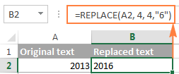
Note. An Excel REPLACE formula always returns a text string, not number. In the screenshot above, notice the left alignment of the returned text value in B2, and compare it to the right-aligned original number in A2. And because it's a text value you won't be able to use it in other calculations unless you convert it back to number, for example by multiplying by 1 or by using any other method described in How to convert text to number.
Using Excel REPLACE function with dates
As you have just seen, the REPLACE function works fine with numbers, except that it returns a text string :) Remembering that in the internal Excel system, dates are stored as numbers, you may try to use some Replace formulas on dates. Results would be quite embarrassing.
For instance, you have a date in A2, say 1-Oct-14, and you want to change "Oct" to "Nov". So, you write the formula REPLACE(A2, 4, 3, "Nov") that tells Excel to replace 3 chars in cells A2 beginning with the 4th char… and got the following result:
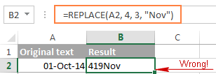
Why's that? Because "01-Oct-14" is only a visual representation of the underlying serial number (41913) that represents the date. So, our Replace formula changes the last 3 digits in the above serial number to "Nov" and returns the text string "419Nov".
To get the Excel REPLACE function to correctly work with dates, you can convert dates to text strings first by using the TEXT function or any other technique demonstrated in How to convert date to text in Excel. Alternatively, you can embed the TEXT function directly in the old_text argument of the REPLACE function:
=REPLACE(TEXT(A2, "dd-mmm-yy"), 4, 3, "Nov")
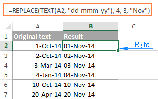
Please remember that the result of the above formula is a text string, and therefore this solution works only if you are not planning to use the modified dates in further calculations. If you do need dates rather than text strings, use the DATEVALUE function to turn the values returned by the Excel REPLACE function back to dates:
=DATEVALUE(REPLACE(TEXT(A2, "dd-mmm-yy"), 4, 3, "Nov"))
Nested REPLACE functions to do multiple replacements in a cell
Quite often, you may need to do more than one replacement in the same cell. Of course, you could do one replacement, output an intermediate result into an additional column, and then use the REPLACE function again. However, a better and more professional way is to use nested REPLACE functions that let you perform several replacements with a single formula. In this context, "nesting" means placing one function within another.
Consider the following example. Supposing you have a list of telephone numbers in column A formatted as "123456789" and you want to make them look more like phone numbers by adding hyphens. In other words, your goal is to turn "123456789" into "123-456-789".
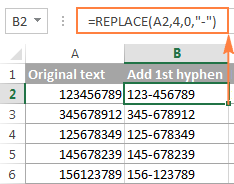
Inserting the first hyphen is easy. You write a usual Excel Replace formula that replaces zero characters with a hyphen, i.e. adds a hyphen in the 4th position in a cell:
=REPLACE(A2,4,0,"-")
The result of the above Replace formula is as follows:
Okay, and now we need to insert one more hyphen in the 8th position. To do this, you place the above formula within another Excel REPLACE function. More precisely, you embed it in the old_text argument of the other function, so that the second REPLACE function will handle the value returned by the first REPLACE, and not the value in cell A2:
=REPLACE(REPLACE(A2,4,0,"-"),8,0,"-")
As the result, you get the phone numbers in the desired formatting:
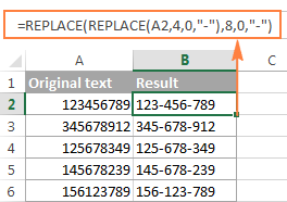
In a similar manner, you can use nested REPLACE functions to make text strings look like dates by adding a forward slash (/) where appropriate:
=(REPLACE(REPLACE(A2,3,0,"/"),6,0,"/"))
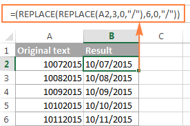
Moreover, you can convert text strings into real dates by wrapping the above REPLACE formula with the DATEVALUE function:
=DATEVALUE(REPLACE(REPLACE(A2,3,0,"/"),6,0,"/"))
And naturally, you are not limited in the number of functions you can nest within one formula (the modern versions of Excel 2010, 2013 and 2016 allow up to 8192 characters and up to 64 nested functions in a formula).
For example, you can use 3 nested REPLACE functions to have a number in A2 appear like date and time:
=REPLACE(REPLACE(REPLACE(REPLACE(A2,3,0,"/") ,6,0,"/"), 9,0, " "), 12,0, ":")
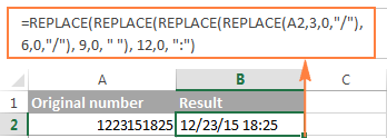
Replacing a string that appears in a different position in each cell
So far, in all the examples we have been dealing with values of a similar nature and have made replacements in the same position in each cell. But real-life tasks are often more complicated than that. In your worksheets, the characters to be replaced may not necessarily appear in the same place in each cell, and therefore you will have to find the position of the first character that should be replaced. The following example will demonstrate what I'm talking about.
Supposing you have a list of email addressing in column A. And the name of one company has changed from "ABC" to, say, "BCA". So, you have to update all of the clients' email addressing accordingly.
But the problem is that the client names are of different length, and that is why you cannot specify exactly where the company name begins. In other words, you do not know what value to supply in the start_num argument of the Excel REPLACE function. To find it out, use the Excel FIND function to determine the position of the first char in the string "@abc":
=FIND("@abc",A2)
And then, supply the above FIND function in the start_num argument of your REPLACE formula:
=REPLACE(A2, FIND("@abc",A2), 4, "@bca")
Tip. We include "@" in our Excel Find and Replace formula to avoid accidental replacements in the name part of email addresses. Of course, there's a very slim chance that such matches will occur, and still you may want to be on the safe side.
As you see in the following screenshot, the formula has no problem with finding and replacing the old text with the new one. However, if the text string to be replaced is not found, the formula returns the #VALUE! error:
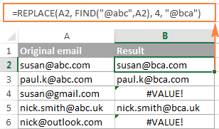
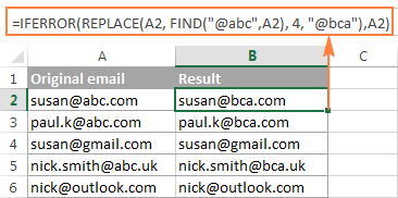
And we want the formula to return the original email address instead of the error. So, let's enclose our FIND & REPLACE formula in the IFERROR function:
=IFERROR(REPLACE(A2, FIND("@abc",A2), 4, "@bca"),A2)
And this improved formula works perfectly, doesn't it?
Another practical application of the REPLACE function is to capitalize the first letter in a cell. Whenever you deal with a list of names, products, and the like, you can use the above-linked formula to change the first letter to UPPERCASE.
Tip. If you want to make the replacements in the original data, an easier way would be using the Excel FIND and REPLACE dialog.
Excel SUBSTITUTE function
The SUBSTITUTE function in Excel replaces one or more instances of a given character or text string with a specified character(s).
The syntax of the Excel SUBSTITUTE function is as follows:
The first three arguments are required and the last one is optional.
- Text - the original text in which you want to substitute characters. Can be supplied as a test string, cell reference, or a result of another formula.
- Old_text - the character(s) you want to replace.
- New_text - the new character(s) to replace old_text with.
- Instance_num - the occurrence of old_text you want to replace. If omitted, every occurrence of the old text will be changed to the new text.
For example, all of the below formulas substitute "1" with "2" in cell A2, but return different results depending on which number you supply in the last argument:
=SUBSTITUTE(A2, "1", "2", 1) - Substitutes the first occurrence of "1" with "2".
=SUBSTITUTE(A2, "1", "2", 2) - Substitutes the second occurrence of "1" with "2".
=SUBSTITUTE(A2, "1", "2") - Substitutes all occurrences of "1" with "2".

In practice, the SUBSTITUTE function is also used for removing unwanted characters from cells. For real-life examples, please see:
Note. The SUBSTITUTE function in Excel is case-sensitive. For example, the following formula replaces all instances of the uppercase "X" with "Y" in cell A2, but it won't replace any instances of the lowercase "x".

Substitute multiple values with a single formula (nested SUBSTITUTE)
As is the case with the Excel REPLACE function, you can nest several SUBSTITUTE functions within a single formula to do several substitutions at a time, i.e. substitute several characters or substrings with a single formula.
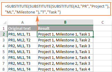
Supposing you have a text string like "PR1, ML1, T1" in cell A2, where "PR" stands for "Project, "ML" stands for "Milestone" and "T" means "Task". What you want is to replace the three codes with full names. To achieve this, you can write 3 different SUBSTITUTE formulas:
=SUBSTITUTE(A2,"PR", "Project ")
=SUBSTITUTE(A2, "ML", "Milestone ")
=SUBSTITUTE(A2, "T", "Task ")
And then nest them into each other:
=SUBSTITUTE(SUBSTITUTE(SUBSTITUTE(A2,"PR","Project "),"ML","Milestone "),"T","Task ")
Notice that we've added a space at the end of each new_text argument for better readability.
To learn other ways to replace multiple values at a time, please see How to do mass find and replace in Excel.
Excel REPLACE vs. Excel SUBSTITUTE
The Excel REPLACE and SUBSTITUTE functions are very similar to each other in that both are designed to swap text strings. The differences between the two functions are as follows:
- SUBSTITUTE replaces one or more instances of a given character or a text string. So, if you know the text to be replaced, use the Excel SUBSTITUTE function.
- REPLACE changes characters in a specified position of a text string. So, if you know the position of the character(s) to be replaced, use the Excel REPLACE function.
- The SUBSTITUTE function in Excel allows adding an optional parameter (instance_num) that specifies which occurrence of old_text should be changed to new_text.
This is how you use the SUBSTITUTE and REPLACE functions in Excel. Hopefully, these examples will prove useful in solving your tasks. I thank you for reading and hope to see on our blog next week!
Download practice workbook
REPLACE and SUBSTITUTE formula examples (.xlsx file)
 by
by
299 comments
Hi, I have want to convert all cases to PROPER except UPPER Case in Single cell.
E:g 1,
From
"uniTed Arab EmiratEs (UAE)"
To
"United Arab Emirates (UAE)"
E:g 2,
From
"i love APPLE"
To
"I Love APPLE"
Any Solution to this ???
Hello
Can Anyone Help Me... I Want Exctract Only "The following manufacturers are covered:" To "Segment by Regions" In between Words seperate And Same as "Segment by Type" to "Segment by Application"
"Solvent Based
Water Based
Hot-Melt-Based"
I want this words separte...
Can anyone Tell me Any Formula...
Unknown is made up of two parts: base material and adhesive. Two or more unconnected objects are connected together by bonding.
The adhesive tapes market in the Asia Pacific region is projected to grow at the highest CAGR.during the forecast period.
Asia Pacific is the fastest-growing market for adhesive tapes
At company level, this report focuses on the production capacity, ex-factory price, revenue and market share for each manufacturer covered in this report.
The following manufacturers are covered:
3M
TESA SE
LINTECORATION
Segment by Regions
North America
Europe
China
Japan
Segment by Type
Solvent Based
Water Based
Hot-Melt-Based
Segment by Application
Packaging
Healthcare
Thank You....
How to replace to another sheet cell by putting value to current cell?
Svetlana -- your blog is one of the most helpful and straightforward around! You provide crystal clear explanations and illustrations, of multiple ways to achieve the same thing... while not burying the easiest solution. Thank you SO much for all your wisdom and work!
Zach: =SUBSTITUTE(B2, ",",".")
Sunil: =SUBSTITUTE(B2, "18-043-","")
Del: =SUBSTITUTE(B2, "$100.00"," ")
Mike: Among your options are the 3 below. The first 2 would return the email address or term of your choice . Then you could filter to show only rows that aren't blank, and delete them. The 3rd shows the word "send" if the item isn't in the list already mailed to.
=IF(ISERROR(INDEX($D$2:$D$499,MATCH($B2,$D$2:$D$499,0))),"",INDEX($D$2:$D$499,MATCH($B2,$D$2:$D$499,0)))
=IF(ISERROR(INDEX($D$2:$D$499,MATCH($B4,$D$2:$D$499,0))),"","sent already")
=IF(ISERROR(INDEX($D$2:$D$499,MATCH($B3,$D$2:$D$499,0))),"send","")
Hello, I am trying to find an easy way to remove some characters from an excel string. For example, it reads - 1st(sp)15.255(sp)$100.00(9sp)Name - where sp is a space. I want to remove the dollar amount ($100.00) but keep everything else, including the spacing. Any suggestions? Love your website, I have learned so much from it but this one has me stumped. Replace will remove the dollar amount but also everything else behind it. Any help would be greatly appreciated. Thanks.
I am trying to find multiple values in a single column and replace them all without using find/replace one by one. Ex. I have a list of 150 email addresses that have already received a mail merge. Those 150 email addresses are all located in another column in a different worksheet that has thousands of email addresses. How do I search for all 150 that have been sent and replace them with a blank cell?
I like to replace below
18-043-0364-04-622
to
0364-04-622
I am looking to replace a comma in a string of text. The comma may or may not be present so I need to search for it, then if it is present, its location changes depending on the string. Once the comma is located, I need to replace it with a period. I convert all my excel files into .CSV and that comma is messing up my data.
If anyone can help with this I would greatly appreciate it.
Thank you!
I have a spreadsheet that I'm trying to build that allows a cell to have a list to choose from. Once the number has been chosen, it replaces verbiage in another cell. for instance, it the number the tech selects in the title cell is 65337-1, it has a configuration within the cells that changes if they choose 65337-2. Not sure if this possible or not.
Thanks
I want to find and replace a word but the color should not change.
For example,
we have a word "confirm" which is in green color and i should replace this word with the word "request" with the same color. What is the formula?
I am looking for a formula which can work in combination with the IFERROR function. On my spreadsheet, I am getting a #DIV/0 error since one of the cells required for a calculation is containing a zero; so I would like to use the IFERROR function to return a zero in a case of an error; moreover, input another 'manual' formula e.g. cells D3/(N3-O3) to come into action when the cells currently containing zero are replaced with >0 numbers. Is there a way I can do this?
I want the difference between old and new numbers in column c,
in which data in column A gets refreshed every 5mins. column B should be replaced by the old value of column A and difference in column c.
eg-
Time A B C
1.00 1 0 1
1.05 4 1 3
1.10 6 4 2
1.15 2 6 -4
1.20 -5 2 -7
1.25 10 -5 15
I have an database whereby I wish to replace partial text in a string using a vlookup in a table on a separate worksheet as follows:
Worksheet1:
A1: this is a test replacement for MPv3 filename
A2: filex32 exists
Worksheet2: This is where I store a table for looking up exact matches against the field text in Worksheet 1
Table Replacement
====== ================
MPv3 MP3
MPv4 MP4
b@listic balistic
/ {leave it blank}
x32 x86
Ideally a substitute function in Column B fields 1 & 2 would result in the fields as per below:
A1: this is a test replacement for MPv3 filename
A2: filex32 exists
B1: this is a test replacement for MP3 filename
B2: filex86 exists
I assume the calculation to substitute the text in A1 would use a vlookup and substitute function however I can't seem to get the formula correct.
Thanks in advance for your assistance.
Regards,
David
Very useful. Thank you.
Hello:
I have a string such as this: BIS-2018-0006-99049&attachment
Need each row below to add +1 to the 990449 in a batch of say 50
SO next entry BIS-2018-99050&attachment, followed by BIS-2018-99051&attachment,
and so on.
Thank you!
James
Hi there!
Below is my question, I often get confused with formulae so pls help.
I am preparing financials and in YTD November sheet in one of the cells the formula is
='Cons Jul'!B37+'Cons Aug'!B37+'Cons sep'!B37+'Cons Oct'!B37+'Cons Nov'!B37
Now I need to copy this sheet and prepare it till YTD December so the formula would be
='Cons Jul'!B37+'Cons Aug'!B37+'Cons sep'!B37+'Cons Oct'!B37+'Cons Nov'!B37'Cons Dec'!B37
There are a number of cells to be changed manually but can I do it using some other short cut?
Thanks!
Hello Everyone,
I understood the logic of SUBSTITUTE, but what if I want to replace more than one digit ?
For example,
DENIZ_13579-ISTANBUL
When I formulate SUBSTITUTE(A2;"1";"") it takes 1 out, that's easy.
My question is, how can I take all the digits out ?
and then in another cell only show those digits 13579 ?
I will appreciate your help
Cheers
Hello, Deniz:
There are several different methods for extracting numbers from a text string. Here's one.
Enter this formula in a blank cell and then with the cursor somewhere in the formula in the formula bar simultaneously press CTRL-Shift-Enter. It's an array formula so it needs the curly brackets around the entire formula which must be entered by simultaneously pressing CTRL-Shift-Enter.
Replace each instance of C30 with the address of the cell where your text string is stored.
=MID(SUMPRODUCT(--MID("01"&C30,SMALL((ROW($1:$300)-1)*ISNUMBER(-MID("01"&C30,ROW($1:$300),1)),ROW($1:$300))+1,1),10^(300-ROW($1:$300))),2,300)
It has the following caveats:
- The input string in cell C30 must be shorter than 300 characters
- There must be at most 14 digits in the input string. (Any following digits will be shown as zeroes.)
-This formula extracts the numbers as text into the cell in which it is entered. If you need the numbers as numbers then use the VALUE function in another cell that references the cell the numbers displayed as text are in.
It will also handle the following two cases correctly:
- If there is a "0" as the first digit of the original string it will be shown correctly in the output
- An input without any digits at all will display an empty string as output (rather than 0).
Hi,
I have imported information form the internet into excel and it keep updating as intended. The problem for me is that i can use whats being imported to multiply with. eks : 8.214605. This will only work if its a comma instead.
So everytime it does a new update, the number change and . comes back.
Any way of making a 2nd cell that changes out the . for a , ?
Great info! I need to convert the first example to second example.
34 59 48.29195(N)
34° 59' 48.29195" N
(so adding the characters in position 3, 6, 15 then replacing first "(" with a space and deleting second ")"
I am not an excel guru and I tried using the replace and substitute command but just could not figure it out :( Any help will be appreciated.
Im not an excel guru neither but i think changing the format of the number from general to something else that may solve this will be good. Perhaps creating a custom format might help hopefully.
Hi
My formula takes a letter designation for the location of the file and replaces with the actual server address. My issue becomes some laptops will actually add the server address instead, I would need to remove it because a VBA adds the static server address. How can I add this possibility with a logic statement to look and remove if present?
if i have two columns A and B with different values in n rows
and i want to replace the column A values with column B values - if the value in column A is less than value in column B
What function should i write
A B
4 8
7 2
n rows
etc
want the 7 to replaced by 2 and so on in other rows till n row
what function should i write
thanks and best wishes
+ryan
Ryan:
Your request is unclear. You write, "I want to replace the column A values with column B values - if the value in column A is less than value in column B." Yet your example is the value in column A is greater than the value in column B.
I'll go with the example. Where the data begins in A2:B2
the formula looks like: =IF(A2>B2,B2,"T")
Enter this in C2 and copy it down the column.
You didn't specify what happens if A2<B2 so I just wrote a "T". You may want to put in something different.
I have an address problem. In these examples:
P.O. Box 851
23 Green St. LOT 214 A
414 Aptitude Way
616 Camelot Dr.
5 Cook St. APT F 5
817 South St. LOT 52 B
44 Quarry Rd. BOX 24 C
My vendor's software drops the last letter or number after "APT", "LOT", or "BOX" because of the last space. If I give them LOT 52B or BOX 24C it prints correctly. The abbreviations APT, LOT, and BOX will always be capitalized. How do I cut the last space in these strings?
Thanks alot bro!!
Heyy, I have to create an equation for if the numbers used is more than 5000, then subtract 5000 from it. then from that derived number,i need to find 8% of it. Of course i tried =IF(B3>=5000,B3-5000*8%). this gets me a higher answer than if i were to do it with a calculator. Can you please help asap please??
Dinesh:
Try this:
=IF(B3>=5000,(B3-5000)*.08,"Value in B3 is Less Than 5000.")
It reads, If B3 is greater than or equal to 5000 then subtract 5000 from the value in B3 and then multiply that remainder times .08 otherwise display a message letting the user know that B3 is not greater than or equal to 5000.
Hi,
7/8/123
88/45/21105648/16455641
456487/6459/54654559/634965/464546/2616
.1/1/1
how do I replace every second /from the above content by using furmulla.
please suggest.
Amar:
I think this is what you're looking for.
Where the data is in A3 and you want to substitute nothing for the second occurrence of the forward slash try this:
=SUBSTITUTE(A3,"/","",2)
Doug
Very helpful tip. Thank you.
I have a small problem..
I have cells that contain several of the same character '_'(quantity varies) and the text 'Category', I wish to remove all the occurrences of '_' along with each 'Category'
Cells contain a1 abc_abcc_defg_category
a2 de_a_category
a3 ghi_cc_126_category
I wish cells in b1 abc abcc defg
b2 de a
b3 ghi cc 126
I've tried several combinations of substitute, replace, match but with no luck. HELP
kindly try below formula for this:-
SUBSTITUTE(SUBSTITUTE(A3,"_"," "),"category"," ")
Please keep your text in cell a3.
Create Excel rule for automatic text / number replacement
I want this to be a rule, so I can just type / enter the team number in the next time and it will automatically replace it with the name of the team.
How to swap alternate characters of the contents of a cell in Excel. Example - A cell containing string 123456 should be converted into 214365 and the result placed in another cell.
Tine:
Because the data is not structured consistently it would not be possible to do what you want. In other words, you need to work the data so that there is a "/" in every place you want a break. I put a "/" at the places in the data to achieve what you wanted.
First, I put the cleaned and formatted data in G30 and entered this formula into J30.
Second, I entered this into K30 =LEFT(G30,FIND("/",G30)-1)
Third, I entered this into L30 =LEFT(J30,3)
Fourth, I entered this into M30 =CONCATENATE(K30,"/",L30)
Because of what you want it will take several steps to get you there, but you'll get there.
Hi,
Does anyone have a consistent way to change/replace the following
Bouvier/Antoine --> Bouvier/Ant
Paitard Xavier --> Paitard/Xav
Di Folco/Marc --> Difolco/Mar
De La Reveliere/Patr --> Delareveliere/Pat
Kinzelin/Marie Helen --> Kinzelin/Mar
Ray Jean Pierre --> Ray/Jea
The result should be lastname/3-letters of first name ...
Thanks for your help!
Regards
Tine
Hello sir
My sentence is
Vishal is a good good good boy
And i want change 2nd "good" into "bad" with subsitute formula can u suggest corret way
Hi team,
I am trying to find a way to convert the following dataset to numbers.
eg.
apple banana orange
orange apple banana
banana orange apple
Where,
apple = 1
banana = 2
orange = 3
So, I want to end up with
1 2 3
3 1 2
2 3 1
Any ideas other than using the Replace All button?
Hi Erin,
If you want to display the number equivalents of your text values in the same cells, I'm afraid you will need to use a special macro to achieve this result or keep on using the standard Excel Find and Replace feature.
However, if we suppose that your table with the text values is in A1:C3, and the table with the number equivalents is in A5:B7, then you can try to enter the following formula, for example, in cell E1:
=INDEX($A$5:$B$7,MATCH(A1,$A$5:$A$7,0),2)
After that copy this formula to the adjacent columns and rows. And then you can select the table with the numbers you've got, press Ctrl + C to copy the selection into the clipboard, select your original dataset and use the Paste - Paste Values option to replace the text with the numbers in the original table.
If your dataset is quite large though, using a macro will be the best option for you. You can search for it in VBA sections on mrexcel.com or excelforum.com.
{A:CM06ICIC0SF0001RBIP0NEFTSC1220ALJOEUREWKJLESUKOWEUJKD00NRIDF;DLJFJ20171128 1636}
In this, need to replace Second character A not entire A letter
For instance, I want to change list of numbers that contains first digits of 081 to 234 but some of the digits also have their last numbers as 081. How do I go about it?. Example : Wish to change the first (081) 08130552081 and not the last to 234
Hi How do i do 1234 to 1324 using formula?
=replace(select word,1,4,"1324")
In using the substitute function, when I add an instance number it gives me the #VALUE! error ?? If I omit the instance number it substitutes all instances with no error ??
Thanks
Found the cause of the error: should not check the "Transition formula evaluation" in the Advance Options.
Hope this help.
Hi Team,
Can some one please help me with this substitute formula?
=SUBSTITUTE(SUBSTITUTE(A96,"9(","DECIMAL("),")",",0)")
this is my input[S9(10) Packed Decimal]and it gives output as SDECIMAL(10,0)
now i want to update this same formula to get the below result
[S9(4)V9(2) Packed Decimal]=DECIMAL(5,2) how can i modify this?
i know this is a silly question but i am new to excel :(
Hi,
does substitute leave non matching substrings within a cell unaltered?
Regards,
Ian
I have four columns of data (A1,B1,C1,D1) - each of which contains either "Y", "N" or is left blank. Any number of cells may be blank or none may be blank. I've used Concatenate to put the string together and, based on the result and a series of IF statement, I render a text string result in another column. For example, "YYYY" = "Good", whereas "NNNN" = "Bad". All well and fine but due to the potential blank cells - the string doesn't properly reflect my options. Essentially I'm expected to derive the result based on a four character string from these Y or N inputs. All I really want to do is consistently replace a blank with a "N", so I can get my four character string and do the final rendering. I want to use only Excel formulas and I think Substitute could be used in combination with Concatenate (and the IF statements) to get me where I need to go.
=SUBSTITUTE(SUBSTITUTE(SUBSTITUTE(SUBSTITUTE(B2,"A","B"),"B","A"),"C","Z"),"Z","C")
can someone please help me on this.
results: "B" is replaced with "A"
"Z" is replaced with "C"
But "A" isn't replaced it stays the same and neither does "C".
I guess u should use if function rather then subsitute. because this funtion is working as first come first serve basis.
HOW TO REPLACE ALL CELLS
original replace
307(306) 307
304(305) 304
300(303) 303
AT SINGLE TIME HOW TO REPLACE PLEASE SUGGEST
=left(a2,find("(",a2)-1)
I have a giant column that lists various dates and includes a time.
I want to delete the comma and the time- leaving only the date.
example:
10/15/12, 5:21 PM
I want to change to:
10/15/12
or in the same column:
1/4/13, 5:40 PM
I want to change to:
1/4/13
I ultimately want to sort the column by date. But without removing the comma and time I cannot get the column to sort by date correctly. Currently the years do not descend correctly.
Thanks in advance for any help!
Hello,
Please try to do the following:
- Select the column with the data you want to modify;
- Press Ctrl + F and go to the “Replace” tab;
- Enter “,*” in the “Find what:” field, and leave the ”Replace with:” field blank;
- Click on the “Replace All” button.
Hope this will help you.
if in cell a2=1/04/2018 apply this formula
=left(a2,find(",",a2)-1)
if in cell a2=1/04/2018,05:14 apply this formula
=left(a2,find(",",a2)-1)
Hi I'm trying to remove quotation marks with the substitute formula but i am getting stuck. Is there a formula to get the following result.
Text Result Needed
b" Note Note
Since excel is not accepting quotation marks in the formula, im getting really confused. thanks for the help.
Hello,
Please try the following formula:
=SUBSTITUTE(A1,"b"&CHAR(34),"")
Hope it will help you.
I have a formatted number say 1523.15 to 1 523.15
I can't add with it how do I take it out?
The space between the 1 and 5 is not a " ", so substitute(1 523.15," ", "") did not work. BTW the formatting was done in VB6 by format(1523.15,"###,###.##")
Hello Hans,
Please try the following formula:
=VALUE(A1)
Where cell A1 contains the formatted number - 1 523.15.
Hope it will help you.
Hello,
I have data in columns as below
1 xyz abc t.u sfd
2 a.b mnn jjj i.j
3 jjj i.o cdf o.p
I need to replace cell which does not contain '.' with 'NA'. as below..
1 NA NA t.u NA
2 a.b NA NA i.j
3 NA i.o NA o.p
Finally I need to arrive at something like below.
1 t.u
2 a.b i.j
3 i.o o.p
Help me on this pls.
hi,
i need this MWCU 677.352-8 need to come MWCU6773528
if possible I would like to strip everything and get the Order ID. the problem is : Location of the order id and sometime it begins with A or 1. Cell Example A1: {"Ref":"bad order","OrderId":"ABSER27"} Cell Example A2: {"OrderId":"ABSER27"} Cell Example A3: {"order_id":"12345678","customer_email":"BADORDER@gmail.com"}
Desired result: B1 = ABSER27 Desired result: B3 = ABSER27 Desired result: B3 = 12345678
I have a column of scanned numbers in column "A". some of these numbers are repeated several times down column "A". I need these numbers in column "A" to be changed to a predetermined part number in column "B" every time they appear eg:
A B
Code Part Number
45627 7yh7895
214789 4hj21345
496581 65753p
45627 7yh7895
45627 7yh7895
214789 4hj21345
45627 7yh7895
Can this be done using substituent& replace function in excel.
Thanks for your assistance
My previous question didn't read as I would've liked
The first 3 things are in column F: then the substitution (where 23 subs in for 14) is in column E. With the subsequent chance with 23 subbing in for 14 (I have that backward in my pervious question. With the new list (with 23 in and 14 out) now in the F column.
So column E would read:
E2: whatever
E3: whatever
E4: whatever
E5: sub in 23
E6 sub out 14
column F would read:
F2: (1, 2, 14, 32, 55) (this is the starting list which is provided)
F3: either the list again or blank, it doesn't matter which
F4: same as F3
F5: (1, 2, 23, 32, 55) this could happen in F5 or F6 it wouldn't matter, but I would want excel to recognize the 23 in and 14 out and make the change in column F.
Is that possible? If so what is the most efficient way to do it?
Thanks for your help.
Kevin