Google Sheets COUNTIF is one of the easiest functions to learn and one of the handiest to use.
It's time to pick up some knowledge on how COUNTIF is used in Google Spreadsheet and learn why this function makes a true Google Spreadsheet companion.
What is the COUNTIF function in Google Sheets?
This short helper allows us to count how many times a certain value appears within a specified data range.
COUNTIF syntax in Google Sheets
The syntax of our function and its arguments are as follows:
- range — a range of cells where we want to count a certain value. Required.
- criterion or searching criterion — a value to find and count across the data range indicated in the first argument. Required.
Google Spreadsheet COUNTIF in practice
It may seem that COUNTIF is so simple that it doesn't even count as a function (pun intended), but in truth its potential is quite impressive. Its searching criteria alone is enough to earn such a description.
The thing is that we can decide to look for not only concrete values but also those that meet certain criteria.
It's high time to try and build a formula together.
Google Spreadsheet COUNTIF for text and numbers (exact match)
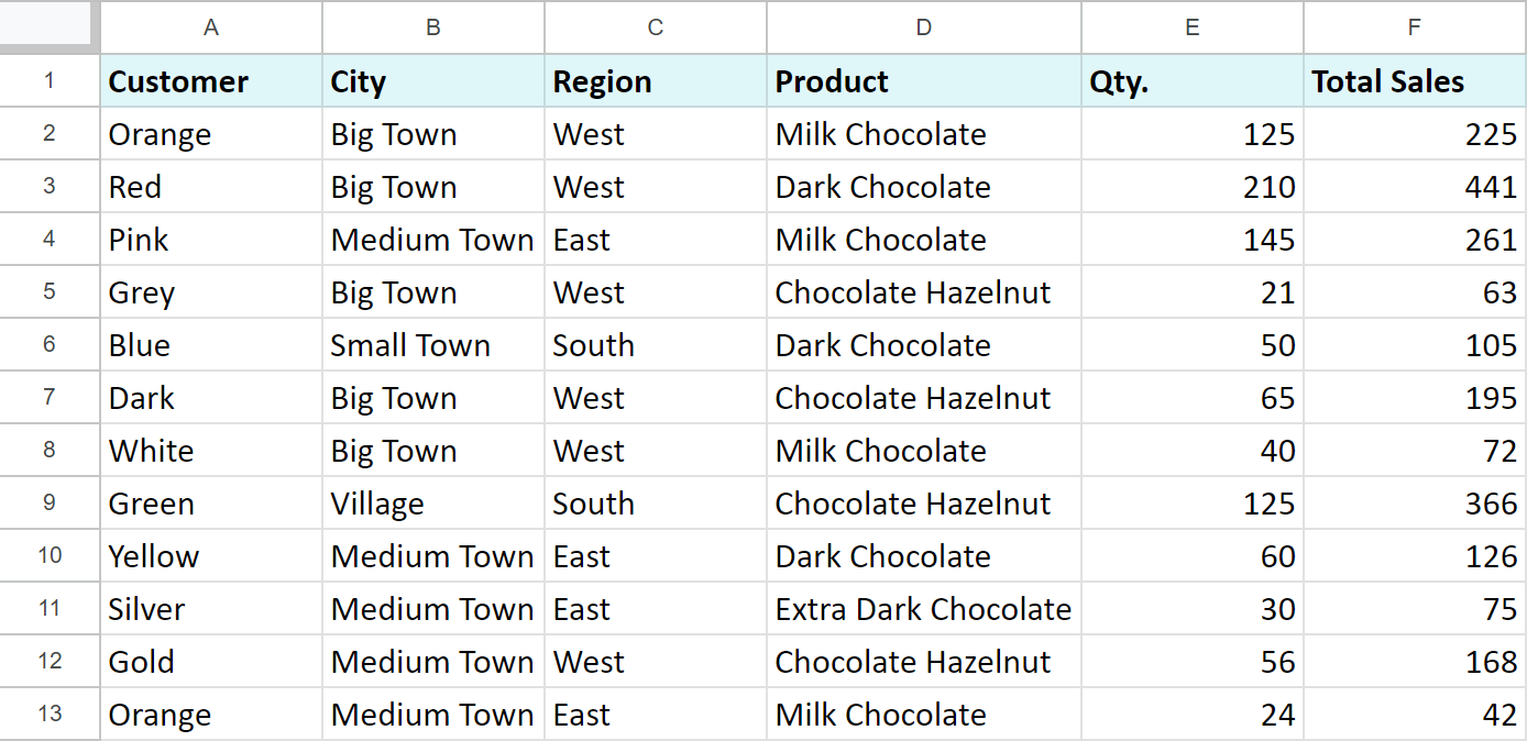
Let's suppose your company sells various types of chocolate in several consumer regions and works with many clients.
This is how your sales data look like in Google Sheets:
Let's begin with the basics.
We need to count the number of "Milk Chocolate" sold. Place the cursor in the cell where you want to get the result and enter the equality sign (=). Google Sheets immediately understands that we are going to enter a formula. As soon as you type the letter "C", it will prompt you to choose a function that begins with this letter. Select "COUNTIF".
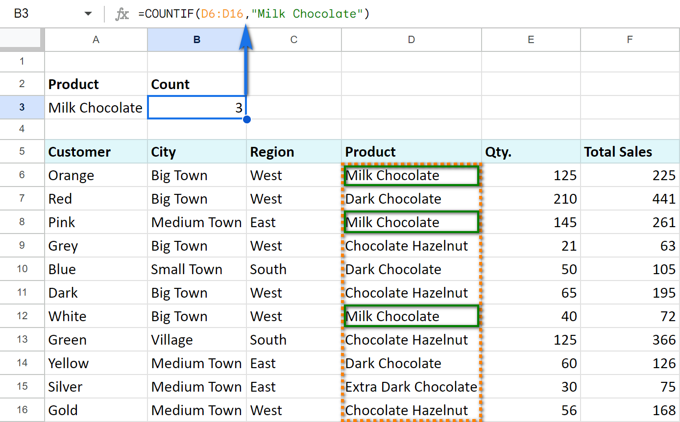
The first argument of COUNTIF is represented by the following range: D6:D16. By the way, you don't have to enter the range manually — mouse selection is enough. Then enter a comma (,) and specify the second argument — searching criteria.
The second argument is a value that we're going to look for across the selected range. In our case it's going to be the text — "Milk Chocolate". Remember to finish the function with a closing bracket ")" and press "Enter".
Also, don't forget to enter double quotes ("") when using text values.
Our final formula looks as follows:
=COUNTIF(D6:D16,"Milk Chocolate")
As a result, we get three sales of this type of chocolate.
Tip. To count words and characters in Google Sheets, visit this tutorial.
Note. COUNTIF function works with a single cell or neighboring columns. In other words, you can't indicate a few separate cells or columns and rows. Please see the examples below.
Incorrect formulas:
=COUNTIF(C6:C16, D6:D16,"Milk Chocolate")
=COUNTIF(D6, D8, D10, D12, D14,"Milk Chocolate")
Correct usage:
=COUNTIF(C6:D16,"Milk Chocolate")
=COUNTIF(D6,"Milk Chocolate") + COUNTIF(D8,"Milk Chocolate") + COUNTIF(D10,"Milk Chocolate") + COUNTIF(D12,"Milk Chocolate") + COUNTIF(D14,"Milk Chocolate")
You may have noticed that it's not really convenient to set the searching criteria in the formula — you have to edit it every time. The better decision would be to write the criteria down other Google Sheets cell and reference that cell in the formula.
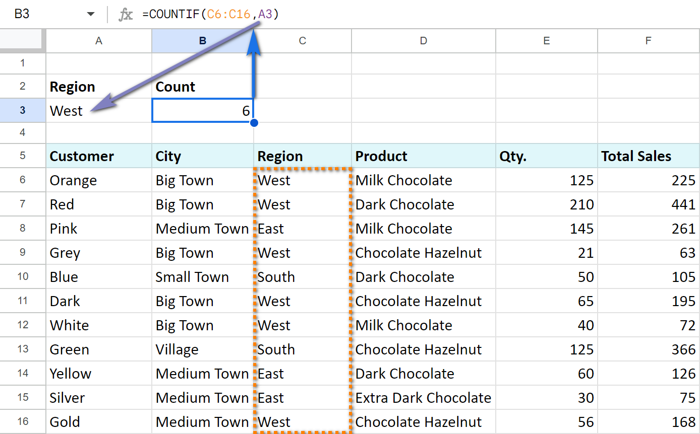
Let's count the number of occurred sales in the "West" region using the cell reference in COUNTIF. We'll get the following formula:
=COUNTIF(C6:C16,A3)
The function uses the content of A3 (the text value "West") in its calculations. As you can see, it's a lot easier now to edit the formula and its searching criteria.
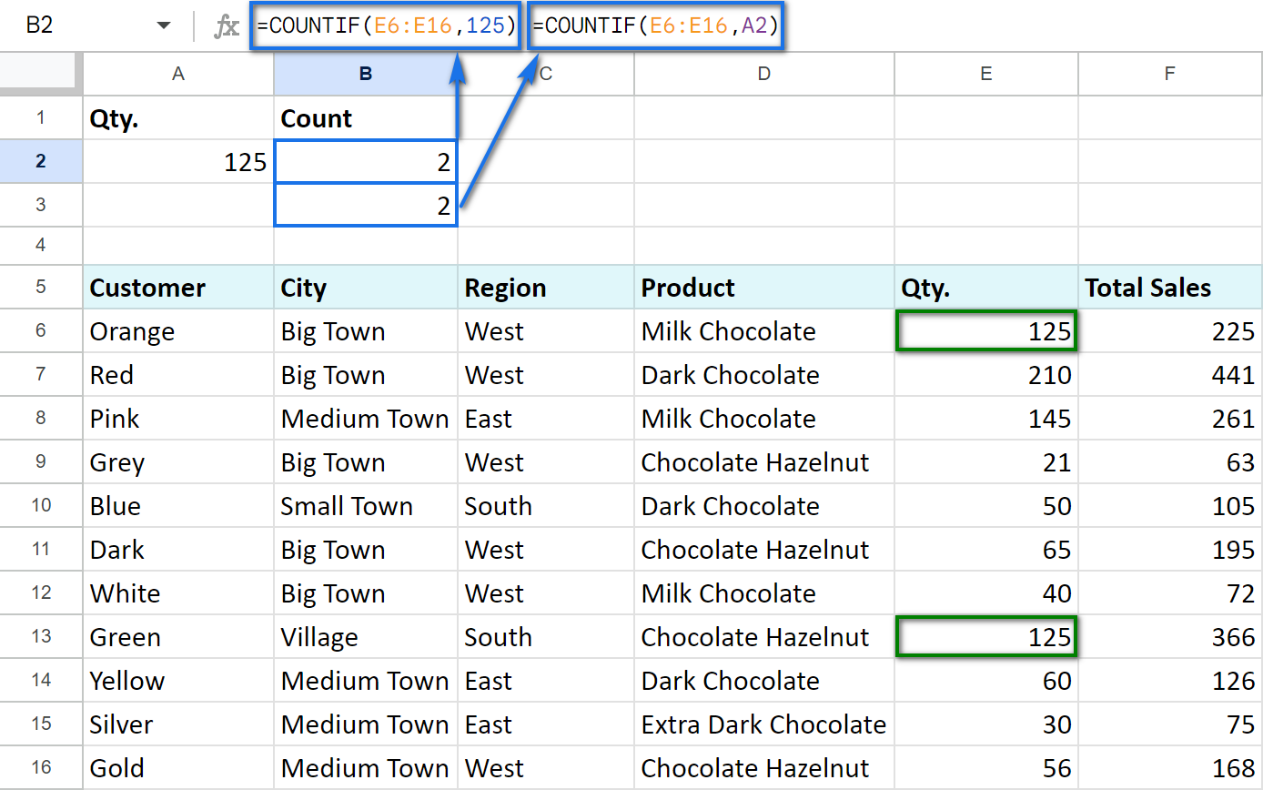
Of course, we can do the same thing with numerical values. We can count the number of occurrences of the number "125" by indicating the number itself as a second argument:
=COUNTIF(E6:E16,125)
or by replacing it with a cell reference:
=COUNTIF(E6:E16,A3)
Google Spreadsheet COUNTIF function and wildcard characters (partial match)
What is great about COUNTIF is that it can count whole cells as well as parts of the cell's contents. For that purpose, we use wildcard characters: "?", "*".
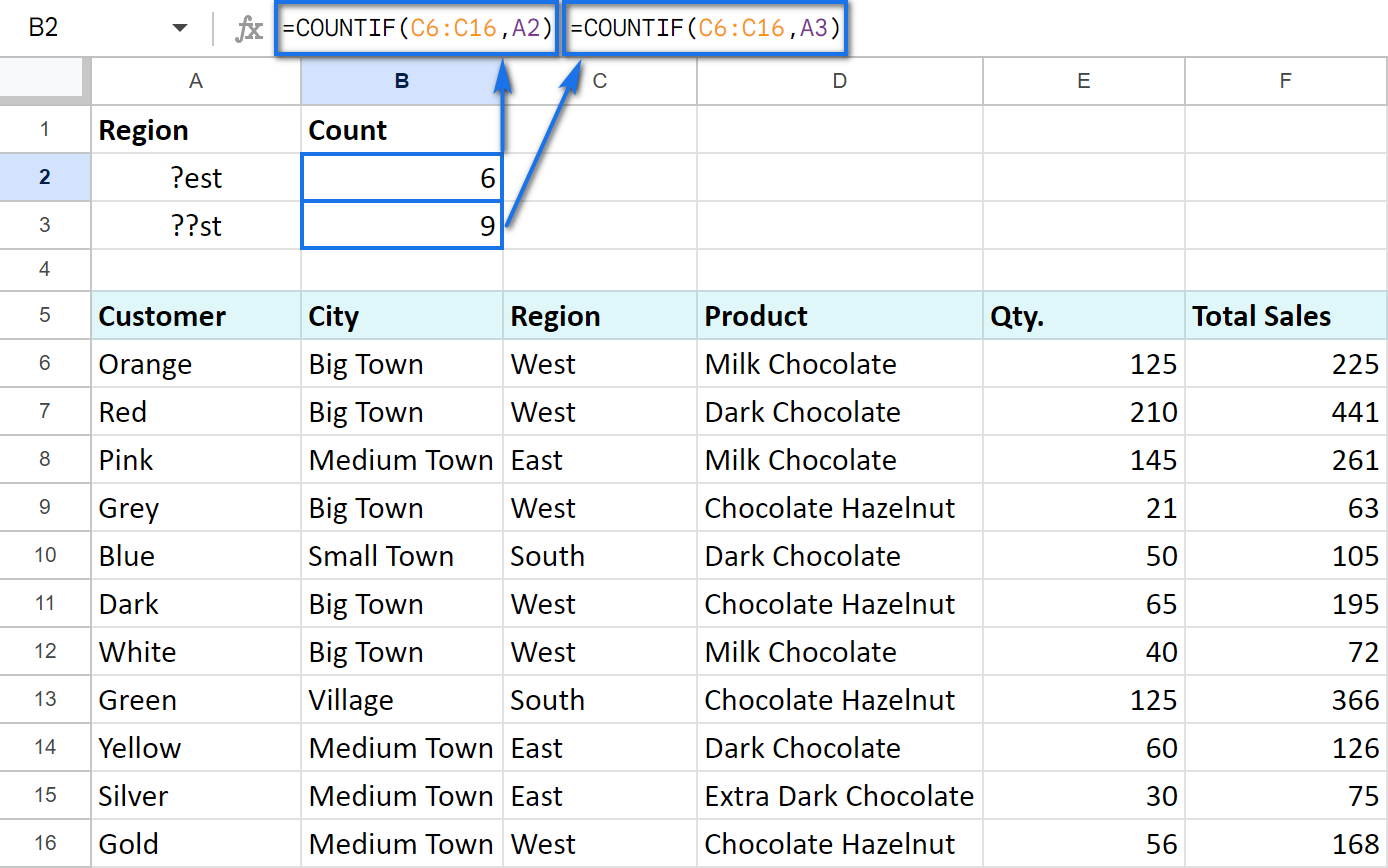
For instance, to count the sales in some particular region we can use only part of its name: enter "?est" into A2. A question mark (?) replaces one character. We are going to look for the 4-letter words ending with "est", including spaces.
Use the following COUNTIF formula in B2:
=COUNTIF(C6:C16,A2)
As you already know, the formula can easily take the next form:
=COUNTIF(C6:C16, "?est")
And we can see 6 sales in the "West" region.
Now let us employ the B3 cell for another formula:
=COUNTIF(C6:C16,A3)
What is more, we'll change the criteria to "??st" in A3. It means that now we are going to look for 4-letter words ending with "st". Since in this case two regions ("West" and "East") satisfy our criteria, we will see 9 sales:
Similarly, we can count the number of sales of the goods using an asterisk (*). This symbol replaces not just one, but any number of characters:
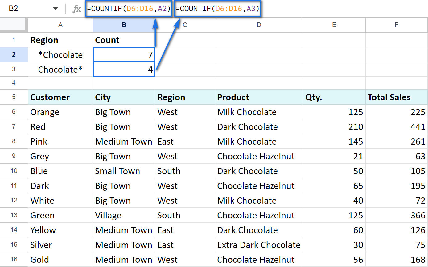
=COUNTIF(D6:D16,A2)
"*Chocolate" in A2 to count all the products ending with "Chocolate".
=COUNTIF(D6:D16,A3)
"Chocolate*" in A3 to count all the products starting with "Chocolate".
And, as you may have guessed, if you enter "*Chocolate*", you're going to look for all the products that contain the word "Chocolate".
Note. If you need to count the number of words that contain an asterisk (*) and a question mark (?), then use tilde sign (~) before those characters. In this case, COUNTIF will treat them as simple signs rather than searching characters. For example, to look for the values that contain "?", the formula will be:
=COUNTIF(D6:D16,"*~?*")
COUNTIF Google Sheets for less than, greater than or equal to
The COUNTIF function is able to count not only how many times some number appears, but also how many of the numbers are greater than/less than/equal to/not equal to another specified number.
For that purpose, we use corresponding mathematical operators: "=", ">", "<", ">=", "<=", "<>".
Check out the table below to see how it works:
| Criteria | Formula example | Description |
| The number is greater than | =COUNTIF(F7:F16,">100") |
Count cells where values are greater than 100. |
| The number is less than | =COUNTIF(F7:F16,"<100") |
Count cells where values are less than 100. |
| The number equals to | =COUNTIF(F7:F16,"=100") |
Count cells where values equal to 100. |
| The number is not equal to | =COUNTIF(F7:F16,"<>100") |
Count cells where values are not equal to 100. |
| The number is greater than or equal to | =COUNTIF(F7:F16,">=100") |
Count cells where values are greater than or equal to 100. |
| The number is less than or equal to | =COUNTIF(F7:F16,"<=100") |
Count cells where values are less than or equal to 100. |
Note. It's very important to enclose the mathematical operator along with a number in the double quotes.
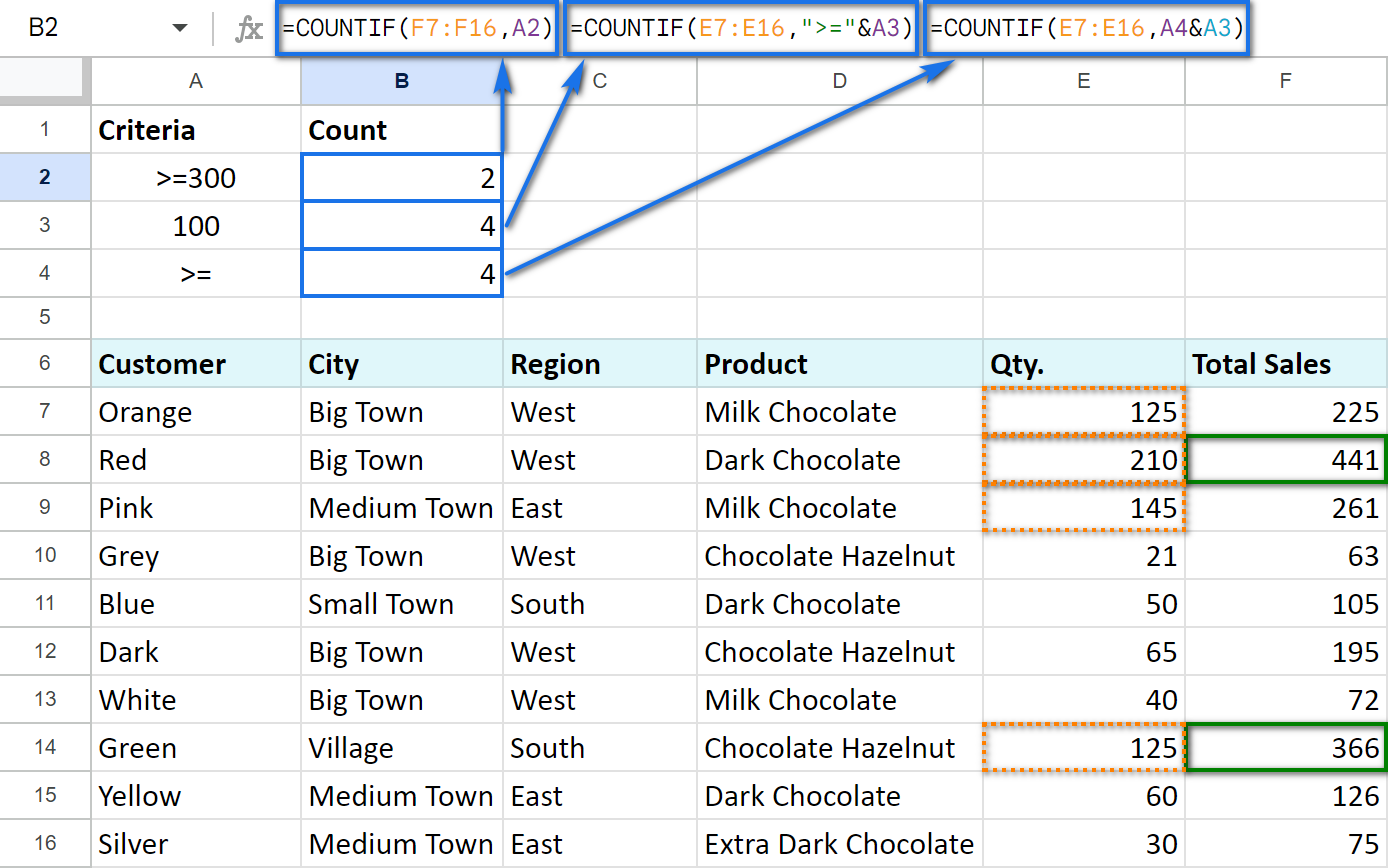
If you want to change the criteria without altering the formula, you can reference the cells as well.
Let me reference A2 and put the formula in B2, just as I did before:
=COUNTIF(F7:F16,A2)
To create more sophisticated criteria, use an ampersand (&).
For example, B3 contains a formula which counts the number of values greater than or equal to 100 in the E7:E16 range:
=COUNTIF(E7:E16,">="&A3)
B4 has the very same criteria, but we reference not only the number in that cell but also a mathematical operator. This makes it even easier to adapt COUNTIF formula if necessary:
=COUNTIF(E7:E16,A4&A3)
Tip. We've been asked a lot about counting those cells that are greater than or less than values in another column. If that's what you're looking for, you will need another function for the job — SUMPRODUCT.
For example, let's count all rows where sales in column E are bigger than in the same row of column F:
=SUMPRODUCT(--(E6:E17>F6:F17))
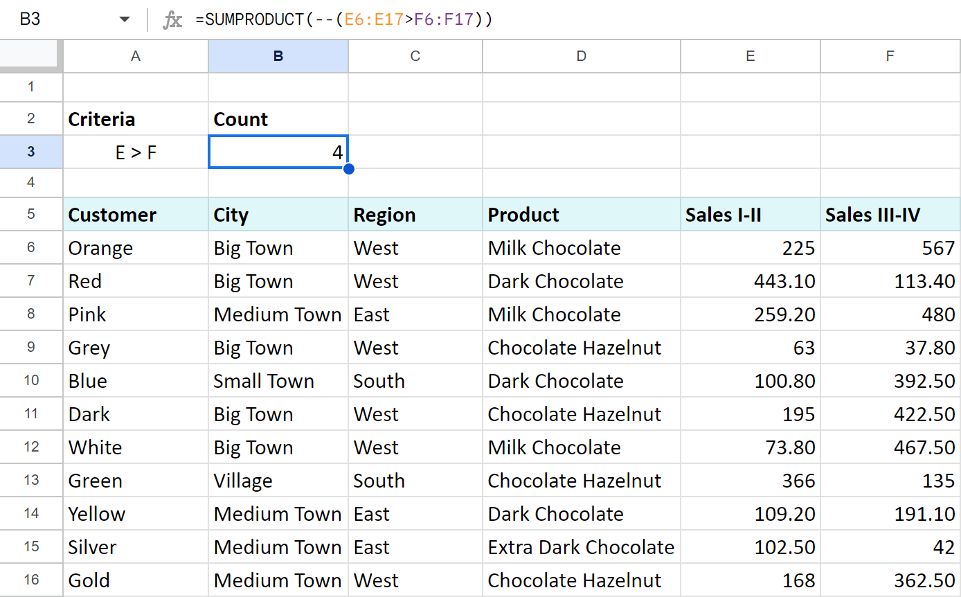
- The part at the core of the formula — E6:E17>F6:F17 — compares values in columns E and F. When the number in column E is greater, the formula takes it as TRUE, otherwise — FALSE.
You'll see that if you enter the same into the ArrayFormula:
=ArrayFormula(E6:E17>F6:F17)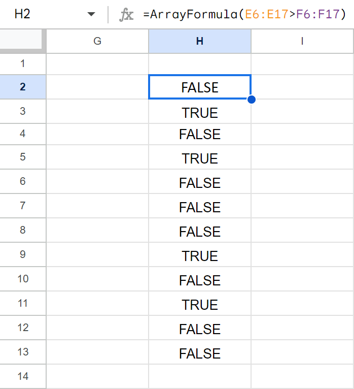
- Then the formula takes this TRUE/FALSE result and turns it into 1/0 numbers with the help of the double unary operator (--).
- This lets SUM do the rest — total the number of when E is greater than F.
Google Spreadsheet COUNTIF with multiple criteria
Sometimes it's necessary to count the number of values that answer at least one of the mentioned conditions (OR logic) or multiple criteria at once (AND logic). Based on that, you can use either a few COUNTIF functions in a single cell at a time or the alternate COUNTIFS function.
Count in Google Sheets with multiple criteria — AND logic
The only way I’d advise you to use here is with a special function that is designed to count by multiple criteria — COUNTIFS:
It is normally used when there are values in two ranges that should meet some criteria or whenever you need to get the number falling between a specific range of numbers.
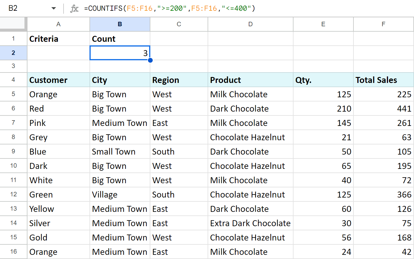
Let’s try and count the number of total sales between 200 and 400:
=COUNTIFS(F5:F16,">=200",F5:F16,"<=400")
Count uniques in Google Sheets with multiple criteria
You can go further and count the number of unique products between 200 and 400.
Nope, it's not the same as above! :) The above COUNTIFS counts each occurrence of sales between 200 and 400. What I suggest is to also look at the product. If its name occurs more than once, it won't be included in the result.
There's a special function for that — COUNTUNIQUEIFS:
Compared to COUNTIFS, it's the first argument that makes the difference. Count_unique_range is that range where the function will count unique records.
Here's how the formula and its result will look:
=COUNTUNIQUEIFS(D5:D16,F5:F16,">=200",F5:F16,"<=400")
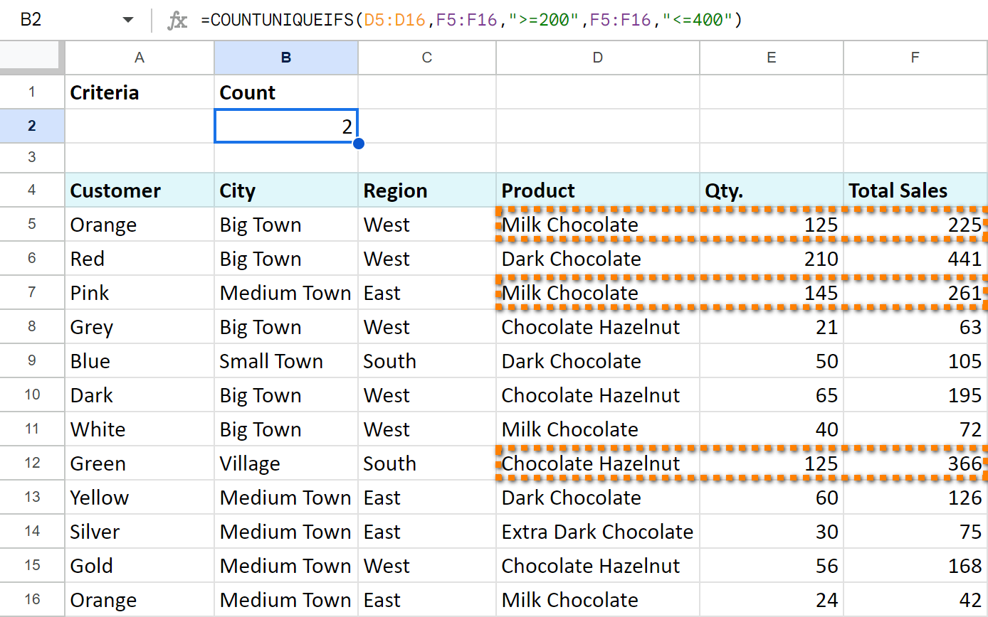
Look, there are 3 rows that meet my criteria: the sales are 200 and greater and at the same time are 400 or less.
However, 2 of them belong to the same product — Milk Chocolate. COUNTUNIQUEIFS counts the first mention of the product only.
Thus, I know that there are only 2 products that meet my criteria.
Count in Google Sheets with multiple criteria — OR logic
When only one of all criteria is enough, you’d better use several COUNTIF functions.
Example 1. COUNTIF + COUNTIF
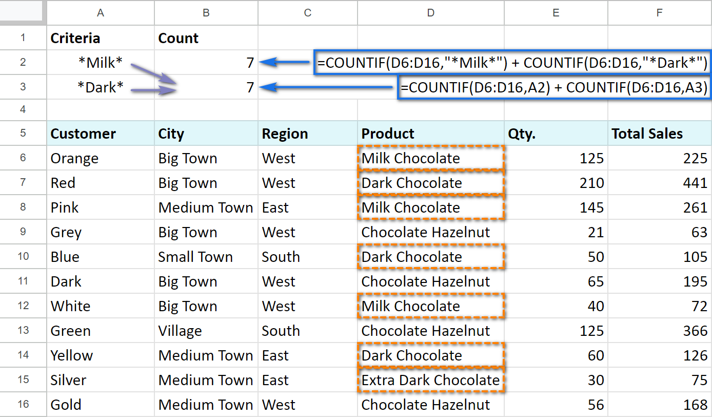
Let's count the number of sales of black and white chocolate. To do that, enter the following formula in B2:
=COUNTIF(D6:D16,"*Milk*") + COUNTIF(D6:D16,"*Dark*")
Tip. I use asterisk (*) to ensure that the words "dark" and "milk" will be counted no matter where they are in the cell — at the beginning, in the middle, or at the end.
Tip. You can always introduce cell references to your formulas. See how it looks on the screenshot below in B3, the result remains the same:
=COUNTIF(D6:D16,A2) + COUNTIF(D6:D16,A3)
Example 2. COUNTIF — COUNTIF
Now, I am going to count the number of total sales between 200 and 400:
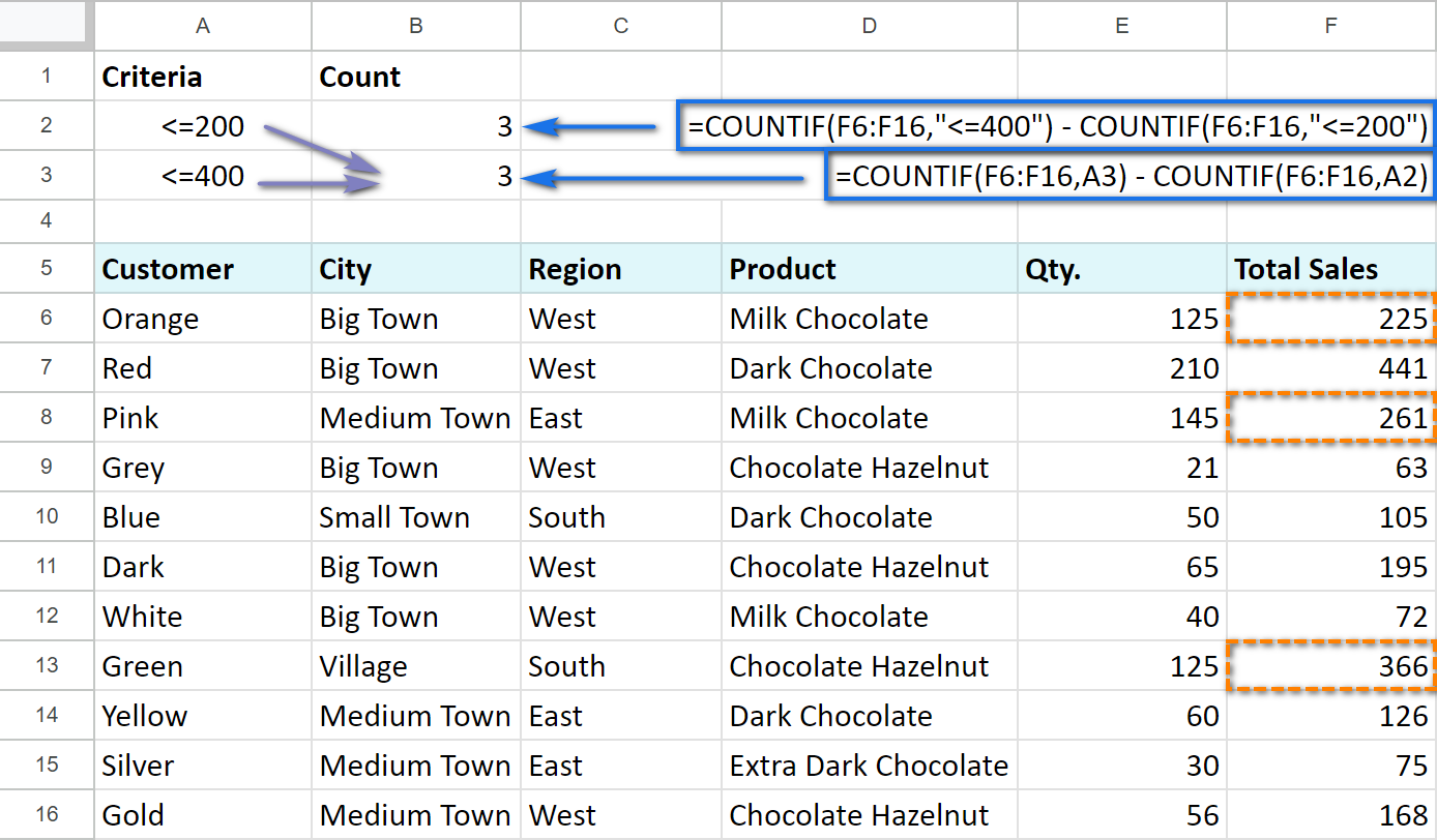
I take the number of totals under 400 and subtract the number of total sales under 200 using the next formula:
=C0UNTIF(F6:F16,"<=400") — COUNTIF(F6:F16,"<=200")
The formula returns the number of sales more than 200 but less than 400.
If you decide to reference A2 and A3 that contain the criteria, the formula will be a bit simpler:
=COUNTIF(F6:F16, A3) — COUNTIF(F6:F16, A2)
A3 cell will have "<=200" criteria, while A4 — "<=400". Put formulas into B2 and B3 and make sure that the result doesn't change — 3 sales over the needed range.
COUNTIF Google Sheets for blank and non-blank cells
With the help of COUNTIF, we can also count the number of blank or non-blank cells within some range.
Let's suppose that we successfully sold the product and marked it as "Paid". If the customer declined the goods, we write zero (0) in the cell. If the deal wasn't closed, the cell remains empty.
To count non-blank cells with any value, use the following:
=COUNTIF(F6:F16,"<>")
or
=COUNTIF(F6:F16,A2)
To count the number of empty cells, make sure to put the COUNTIF formula in the following way:
=COUNTIF(F6:F16,"")
or
=COUNTIF(F6:F16,A3)
The number of cells with a textual value is counted like this:
=COUNTIF(F6:F16,"*")
or
=COUNTIF(F6:F16,A4)
Screenshot below shows that A2, A3, and A4 cells include our criteria:
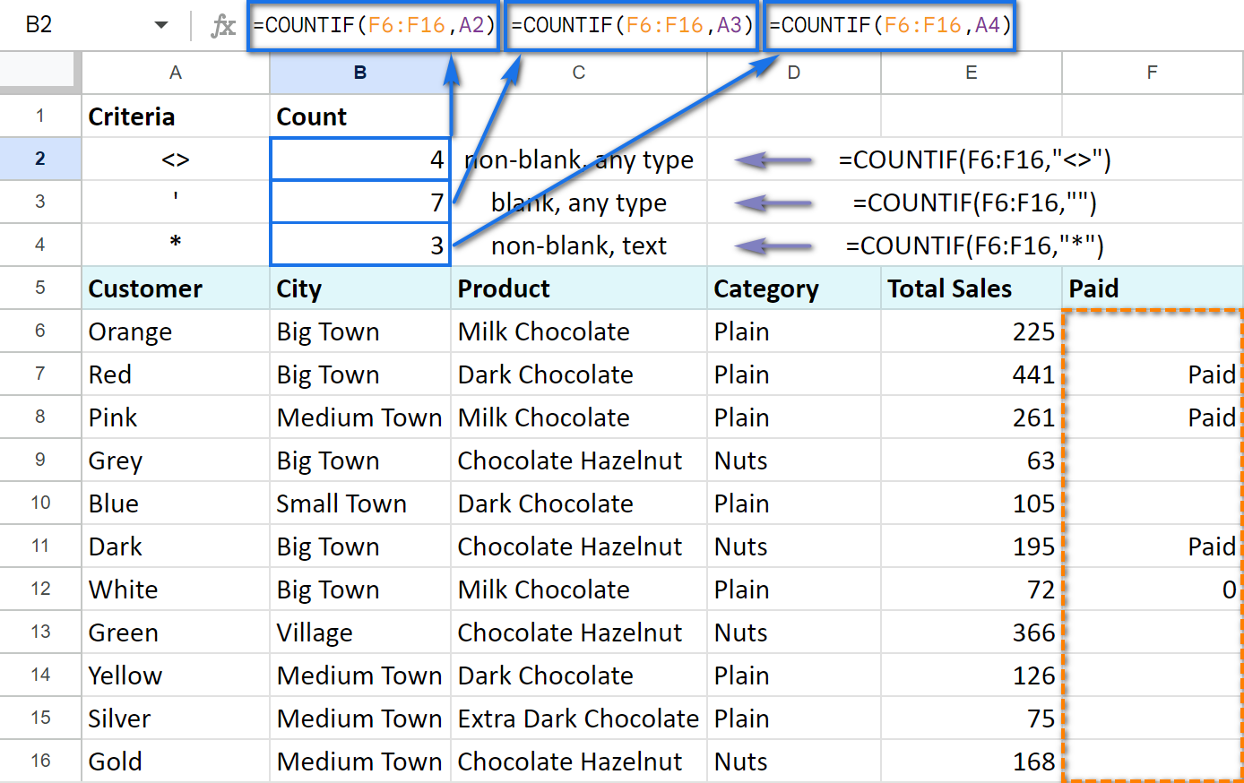
Thus, I have 4 closed deals, 3 of which were paid for and 7 of which have no markings yet and, consequently, are not closed.
COUNTIF and conditional formatting
There is one interesting opportunity that Google Sheets offer — to change the cell's format (like its color) depending on some criteria. For example, we can highlight the values that appear more often in green.
COUNTIF function can play a small part here as well.
Select the range of the cells that you want to format in some special way. Click Format -> Conditional formatting...
In the Format cells if... drop-down list choose the last option Custom formula is, and enter the following formula into the appeared field:
=COUNTIF($B$8:$B$38,B8)/COUNTIF($B$8:$B$38,"*")>0.3
It means that the condition will be answered if the value from B8 appears within B8:B38 in more than 30% of cases:

In a similar way, we add two more formatting rule criteria — if the cell value appears more often than in 25% of cases and more often than in 20%:
=COUNTIF($B$8:$B$38,B8)/COUNTIF($B$8:$B$38,"*")>0.25
=COUNTIF($B$8:$B$38,B8)/COUNTIF($B$8:$B$38,"*")>0.2
Keep in mind that the first criterion will be checked beforehand, and if it's met, the rest won't apply. That is why you'd better start with the most unique values moving to the most common ones. If the cell value doesn't meet any criteria, its format will remain intact.
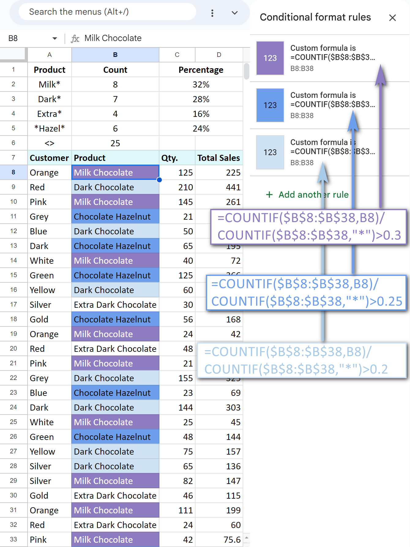
You can see that the colour of the cells has changed according to our criteria.
To make sure, we also counted the frequency of some values in C2:C5 using the COUNTIF function. The results confirm that COUNTIF in formatting rule was applied correctly.
Tip. Find more examples on how to count & highlight duplicates in Google Sheets.
All these function examples give us a clear understanding of how Google Spreadsheet COUNTIF offers multiple opportunities to work with the data in a most efficient way.
COUNTIF color in Google Sheets
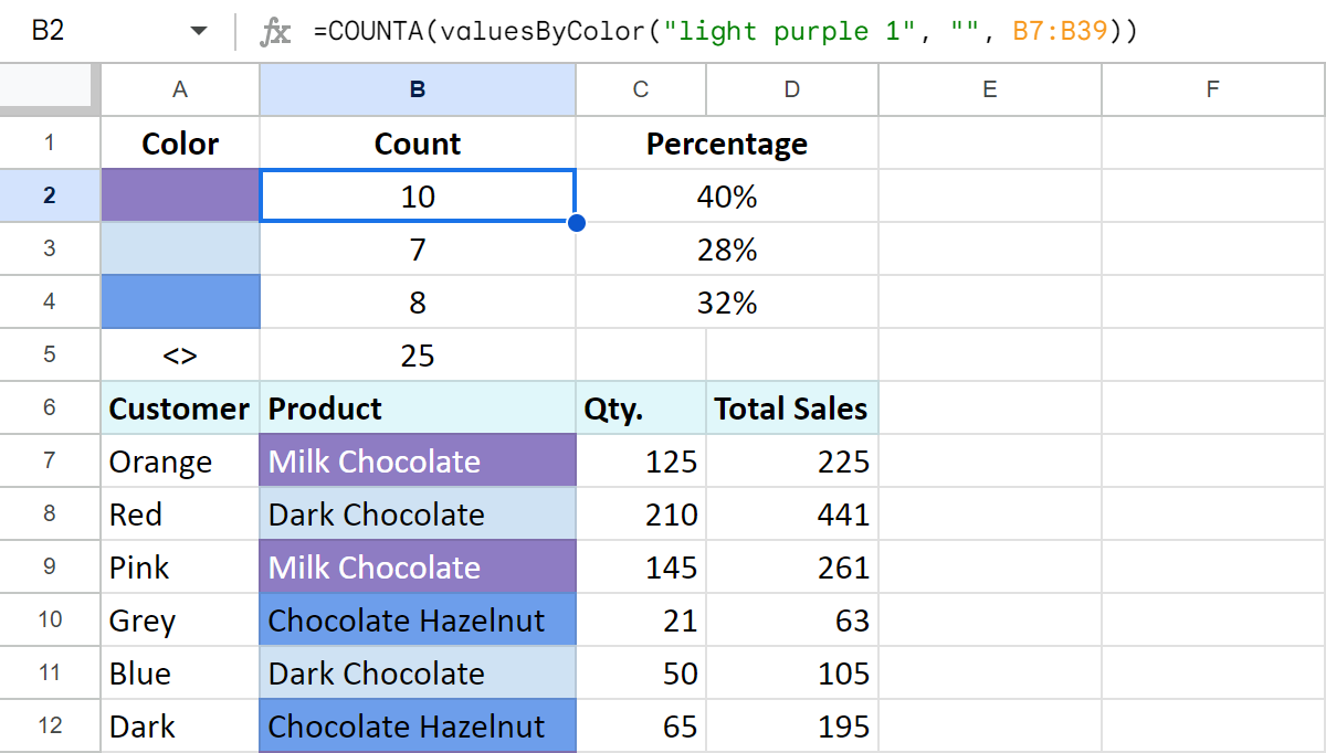
One task that gains popularity is counting cells by their color. Though there's no native Google Sheets function to do that, you can still achieve the result without coding. All you need is an add-on from the Google Workspace Marketplace: Function by Color.
Using the add-on, you will:
- Count cells of any particular font or fill color in your Google Sheet:
- Count all colored cells in the range:
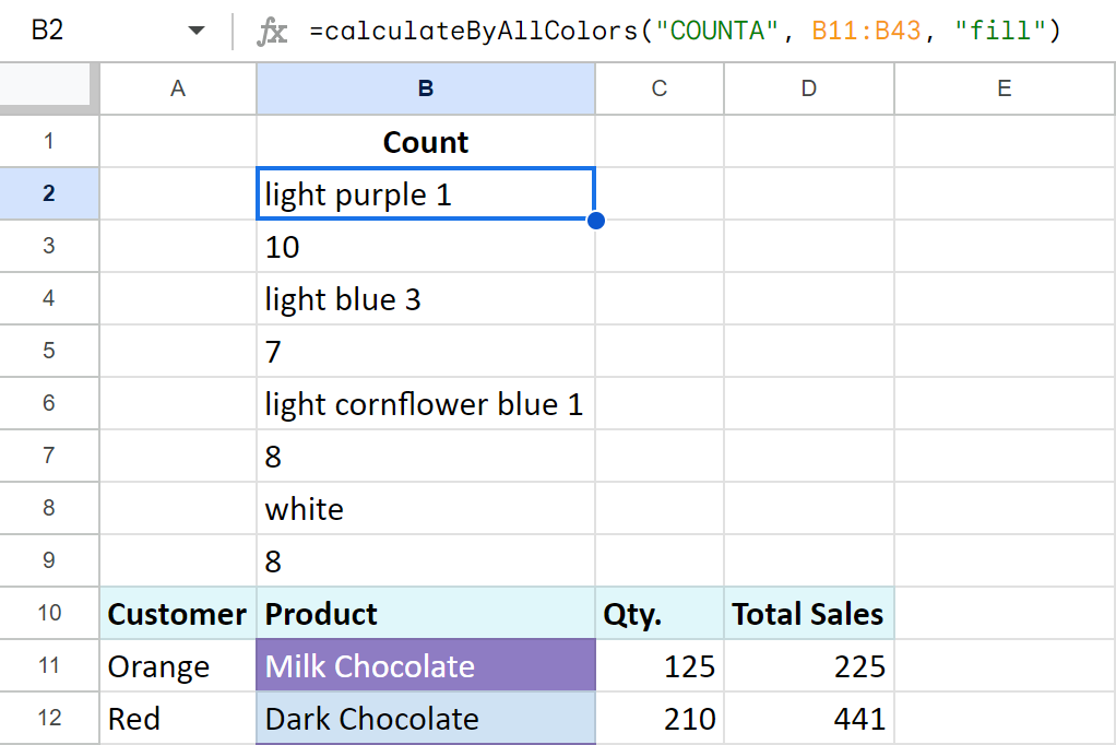
If you're interested in how it works, jump to this article for the details: How to count cells by color in Google Sheets
- Another ability you gain with Function by Color is using colors as extra conditions in your own COUNTIFS (and other) formulas:
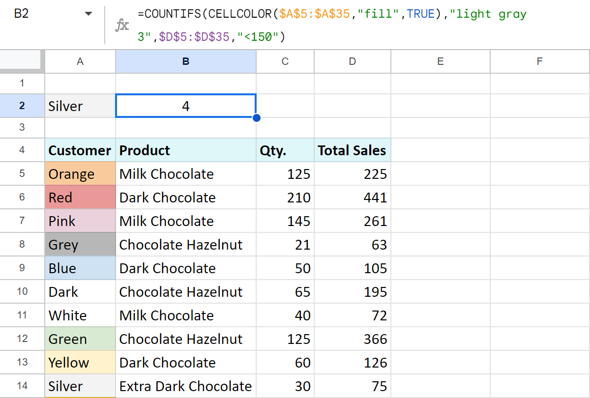
The following blog article breaks down this usage to pieces: Functions for Google Sheets to work with colored cells
Video: How to count colored cells in Google Sheets
Install Function by Color from Google Store to follow the examples along or to try it on your own cases. Let me know how it goes in the comments section below! :)
 by
by 
383 comments
Hi!
Thank you very much for this resource and the amazing job you are doing!
I need your help. I would like to count a number of words in a cell (or a range of cells) but I need to exclude the counting of certain words that are irrelevant (say "a", "the", "and", "an"). The range is the same (say B2:B16), but the criteria of exclusion are multiple. How can I do it without repeating the range every time (in fact, there are a lot more the criteria of exclusion than the four in the example above).
Thank you in advance.
Hi Helen,
Thank you for your lovely words!
As for your task, please share an editable copy of your spreadsheet with us: support@apps4gs.com
I'll check the data you have and see where your criteria are and how many of them you may have. This will help me find the best solution.
Dear Natalia,
Thank you for your reply. I have sent you an example of a neutral text in a Google Spreadsheet and a little comment. Looking forward to reading your comment. Thank you in advance,
Helen
Dear Helen,
Thank you for sharing your spreadsheet. Here's a formula to count all those special words you mentioned:
=COUNT(ArrayFormula(FIND("#", REGEXREPLACE(SPLIT(B3, {" ", ",", ";"}), "^(and|the|a|at|in)$", "#"))))
Subtract this from your total word count and you're good to go :)
I entered the resulting formulas to column E in your spreadsheet, have a look.
In the example below, how would I count the number of shirts of each style, size and color?
Style Size Color
Women's XL Black
Women's XL Black
Men's XL White
Men's 2XL White
Women's XL Green
Men's L Green
Men's 3XL Black
Mens XL Green
Men's XL Black
Women's M Yellow
Women's M Black
Women's XL White
Women's XL Green
Men's XL Black
Women's L Green
Women's XL Green
Men's 3XL Green
Hello Cathy,
if you need to count styles/sizes/colors separately, use COUNTIF as described here.
If you'd like to count based on several conditions at a time, for example, all women's XL black, use COUNTIFS instead.
So trying to add the agent from Column A (9 agents total) to this formula: =ARRAYFORMULA(sum(COUNTIFS(AS2:AS11,{"Yes","VM","No"})))
Hello Kirk,
Sorry but your task is unclear. Could you please describe it in detail?
Hi,
I have calculated how many completed tasks are done in the current day or current month. See below:
=COUNTIFS('Completed Cases'!K2:K5000,">"&TODAY()-1,'Completed Cases'!K2:K5000,"="&EOMONTH(TODAY(),-1)+1,'Completed Cases'!K2:K5000,"<"&EOMONTH(TODAY(),0)+1)
I now need to work out how to break that down and count if the outcome was option A or option B from a different column. What is the best way to do this please?
Hi Ben,
Am I getting it right that some results from K belong to option A from another column and some results belong to B? If so and you'd like to get two different results based on that another column as well, you just neet to have two COUNTIFS formulas where one of the conditions will be for that another column:
=COUNTIFS('Completed Cases'K2:K5000, ">"&TODAY()-1, 'Completed Cases'!K2:K5000, "="&EOMONTH(TODAY(),-1)+1, 'Completed Cases'!K2:K5000, "<"&EOMONTH(TODAY(),0)+1, 'Completed Cases'!ANOTHER_COLUMN, "option A")
If that's not really what you need, please try to describe the desired outcome in more detail.
sample sheet for my query below:
https://docs.google.com/spreadsheets/d/1qjlFW13jRoaHbYk4QtDjQqVGtwpr1OpXSc-Mb61Jmr4/edit?usp=sharing
Hi Jack,
you should use COUNTIFS for your task. I've put an example formula in E2 since it's the only row from your task I understand clearly. Please adjust this formula to use in other rows as you need.
Hi, I had managed it just before your replies and had sent my solution but it appears it did not go through?
Thanks anyway
Hi, I have a sheet with actions on.
On another sheet, I want the number of actions where, on the actions sheet:
- value in column C is the value in column C of the count sheet (e.g. where C9 = C9)
- value in column H of the action sheet is "Strike"
- value in column J of the action sheet is "Active"
How would I achieve this?
Thanks
Hi Jack,
please see my reply to your comment above.
Did it now, thanks anyway.
=COUNTIFS('Log Sheet'!C9:C,C9,'Log Sheet'!H9:H,"Strike",'Log Sheet'!J9:J,"Active")
Hi,
I'm trying to do something similar. Let's pretend on your sample sheet that you had in Column E another list of products. Some said Dark Chocolate, Milk Chocolate, Extra Dark Chocolate, but you also had just plain Chocolate. etc.
I want to be able to count all of the occurrences of Dark Chocolate where (plain) Chocolate would not be counted.
(In my sheet, I need to count all of the occurrences of English 1 separately from all of the occurrences of Honors English 1.
I can get an exact count of all of the "Honors English 1", but anytime I try to count "English 1", because those words also appear in "Honors English 1", it counts both "English 1" and "Honors English 1".
I've linked to a sample sheet: https://docs.google.com/spreadsheets/d/10x13hlqSthvxByNrAqbMSOIM_-VLU6KZ4MdVHkSWa_k/edit?usp=sharing
Hi Elizabeth,
Thank you for sharing the sample right away. I entered the formulas into column J, please take a look. Here's a sample formula:
=COUNTIF($B$2:$E$11,G2)
Hi, is there any possiblitiy for me to use COUNTIFS to count specific text from cell that has Data Validation : drop down list.
Hi Firdauz,
Do you want to take cells with data validation into account or do you want to count text in all items within one data validation in a cell?
How to make a countif to find out amount more than 0:03:00 but lower than 0:04:00
Hello Shen,
You need to use COUNTIFS and list both conditions in the formula. Please see the examples described in this section.
Hi! I created a self-assessment in Google Forms that I'm trying to score with a simple formula. All questions on the assessment have checkbox options for each item, so multiple options can be selected. For example...
For question 1, I choose Options A, B, and D. Option A is worth 1 point, Option B is worth 2 points, and option D is worth 4 points. What formula will take a cell that says 'A, B, D' and calculate 7?
Thanks in advance!
I figured it out this morning. I was overthinking it.
I used =(COUNTIF(cell,"*A*")*1)+(COUNTIF(cell,"*B*")*2)+(COUNTIF(cell,"*C*")*3)+(COUNTIF(cell,"*D*")*4)...
How do i do countif with the power formula?
Hello Olivia,
Sorry, your question is not quite clear, could you please specify?
Hi there,
I am struggling with conditional formatting using custom formula. I want to do a simple formatting into red for all cells in one column that are duplicates (excluding the first occurrence). Following some instructions on the Internet, I select the column (it's formatted as plain text and it only contains numbers) - the range would be A3:A500 (A1 nad A2 are headers) and then Format cells if -> custom formula -> =countif($A$3:$A$500,A3)>1. I also try without $ sign. I also try with (A:A, A3)>1. The problem is that after I have written =countif, no matter what I put there - be it the bracket or whatever - the system highlight this in red and always shows "Invalid formula". Literally, into the custom formula field I can put only: =countif .
I am puzzled and desperate. I have tried on different data in different sheets - same issue everywhere... I would appreciate any help on this matter.
Hi Ela,
First please try to format your data as numbers, not text, before trying to apply the conditional formatting.
If this doesn't help, for me to be able to help you, please share an editable copy of your spreadsheet with us (support@apps4gs.com) with 2 sheets: (1) a shortened copy of your source data (2) the result you expect to get. I kindly ask you to shorten the tables to 10-20 rows. If you have confidential information there, you can replace it with some irrelevant data, just keep the format.
Note. We keep that Google account for file sharing only and don't monitor its Inbox. Please do not email there. Once you share the file, just confirm by replying to this comment.
I have multiple conditional formatting in a google spreadsheet. An example is: =AND($B2="In",COUNTIFS($D:$D,$D2,$B:$B,"In")=6)
This will look at multiple cells and highlight a row based upon the criteria. Each conditional formatting is the same just the number at the end changes which, in turn, highlights the cell a different color. I need to add in another factor to this formatting that if something is column E is indicated as either MEDICAL APPOINTMENT or ILLNESS that is does not count as one of the quantities.
For example is someone has 5 that are marked "In" generally it would highlight all that person's lines purple; however, if 1 of those "INs" are due to a medical appointment or illness it needs to not be counted as 5 INs". but 4 "INs" and highlighted a different color
Hello Shawna,
For me to be able to help you, please share an editable copy of your spreadsheet with us (support@apps4gs.com) with 2 sheets: (1) a shortened copy of your source data (2) the result you expect to get. I kindly ask you to shorten the tables to 10-20 rows. If you have confidential information there, you can replace it with some irrelevant data, just keep the format.
Note. We keep that Google account for file sharing only and don't monitor its Inbox. Please do not email there. Once you share the file, just confirm by replying to this comment.
Hello.
I have a series of cells each containing a 0 or a 1. I would like to count the number of cells containing a 1, but would the count to stop when the first 0 is encountered.
For example, this row:
1 1 1 1 0 1 1 0 0 1 0 0 0
should produce the count 4.
And this one:
1 1 0 1 1 1 1 1 0 1 1 0
should produce the count 2.
Can this be done with COUNTIF (or perhaps with some other function)?
Best wishes
Hello DB,
Assuming your numbers are in A1:M1, here's a formula to try:
=IFERROR(LEN(LEFT(JOIN("",A1:M1),FIND("0",JOIN("",A1:M1))-1)),COUNT(A1:M1))
Hello!
I am trying to count how many values in a column are bigger than the corresponding values in another. Specifically, I have one column that lists the scores of a pre-test that students take at the beginning of class and a list of the student's scores on the test they take at the end of the class. I want to count how many of those scores improved, how would I do that?
Thank you!
Hello Robin,
Assuming your scores are in columns A and B, this formula will do:
=SUMPRODUCT(--(B2:B20>A2:A20))
Hi! Can you help in writing a countif function where the cell does not contain "---"
Hi Abraham,
If I understand you correctly, this formula will do the trick:
=COUNTIF(A2:A10,"<>*---*"
I wonder whether the following is possible.
In TAB1, column A has a number of people's names. Column B onwards is then made up of dates and each column records attendance the attendance of the names in column A
In TAB2, column A has the same names. I want Column B to then repeat whatever is in the cell of today's column in TAB1, so if H1 has today's date, then it will give me the attendance of the named person (in A9) in B9 in TAB2.
How do I get column B in Tab2 to pick up the relevant cell from today's column? Is there an appropriate formula?
Thanks in advance for anyone who is able to help!
Hello Jon,
If I understand you correctly, you can try to use IF along with the VLOOKUP function.
In case you're not sure how to use them exactly, please share a small sample spreadsheet with us (support@apps4gs.com) with your sheets and the example you want to get (the result sheet is of great importance and often gives us a better understanding than any text description). I kindly ask you to shorten the tables to 10-20 rows.
Note. We keep that Google account for file sharing only, please do not email there. Once you share the file, just confirm by replying to this comment.
I'll look into your task and do my best to help.
I was wondering given your example sheet above.
If I want to count the amount of Dark Chocolate sold fx.
so sum up all numbers in column total sales where column Product = "Dark Chocolate"
Figured it out ..
=SUMIF(A2:A500,D1,C2:C500)
Where content of D1 would be the value to look for
Hello Peter,
You're right, it's SUMIF that totals numbers. We have a separate blog post devoted to SUMIF, feel free to take a look.
Thank you for monitoring this channel and helping us out.
How can I use COUNTIFS and OR
=COUNTIFS(E35:T35, "Z" OR COUNTIFS(E35:T35, "1" )
Thank you for the feedback, Walter.
You'll find an answer to your question in this part of the blog post: Count in Google Sheets with multiple criteria – OR logic
Hi I want to count only if two criteria are met.
EG Cells in Range A14:A35 = A and Cells in range C:14:C35 = W
I only want a count of 1 if both conditions are met
Thanks
James
Hi James,
You will find examples of how to count by multiple criteria in this part of the blog post.
Hi there,
I was wondering if there was a way to count if one cell is greater than another range. For example I have a set of scores for students in P column (say range P3:P80) and a second set of score in Q column (Q3:Q80). I want to count the scores in Q column IF they are greater than the initial scores, e.g. I want to count the number of students who got a higher score in the second set of results.
Cheers,
Emma
Hi Emma,
Here's a formula for you to try:
=SUMPRODUCT(--(Q3:Q80>P3:P80))
Hi,
I have this Array Formula in my Google sheet:
={{unique(ArrayFormula(text(K4:K2001,"MMMM")))},
{ArrayFormula(sumif(ArrayFormula(text($K$4:$K$2001,"MMMM")),
unique(ArrayFormula(text(K4:K2001,"MMMM"))),$I$4:$I$2001))}}
The dates it is counting starts from August 2020 through to April 2021.
My problem is for any dates not completed in any given month, it is counted in December, this giving an incorrect count.
Any idea how to fix this?
Hi Colin,
We tried to recreate the formula on our side and it works correctly. Please go to File > Spreadsheet settings and specify what locale you have selected there. Also, provide a couple of examples of your dates in cells.
I have a COUNTIF formula but after the count I want it to divide the count by 2
=COUNTIF(E9:E755,"Couple")
How do I add to the formula above to then divide the count by 2?
Hello Marnee,
Here you go:
=COUNTIF(E9:E755,"Couple")/2
Hi,
Workbook 1, Sheet "ABCSCHOOL" itemizes a constantly changing number of students per section, per grade.
Workbook 2, Sheet "ABCSTAFF" totals the numbers of students per section for all grades, in order to determine the amount of staff needed per section for the coming year.
ABCSTAFF currently has cells that contain the current formula:
=IMPORTRANGE("https://docs.google.com/spreadsheets/d/WORKBOOK1","ABCSCHOOL!E90")
I am using the COUNTIF function in ABCSTAFF to count the number of cells that have a number greater than 0. I am not trying to obtain the sum of the numbers in the cells, but rather the number of cells that contain a number. That formula looks like this: =countif(D4:D10,">0")
What I am trying to figure out is:
1. Is there a formula I can use to count a cell twice if the number in it is greater than 8? For example, Assuming range D4:D10 has 3 cells containing numbers 2, 4 and 5 and another cell containing the number 12, I would like the total count to equal 5 cells, as opposed to 4.
2. How would I add that additional formula to the cell that already contains =IMPORTRANGE("https://docs.google.com/spreadsheets/d/WORKBOOK1","ABCSCHOOL!E90")
Thank you.
Hello Denise,
I'm sorry but your task is quite confusing. I just don't see why the count should return 5 if only 1 number is greater than 8, so I'm not sure what to add to the formula. I also don't understand what the cell with the importrange and the count should contain as a result.
For me to be able to help you, please share a small sample spreadsheet with us (support@apps4gs.com) with 3 sheets: (1-2) a shortened copy of your source data (3) the result you expect to get. I kindly ask you to shorten the tables to 10-20 rows. If you have confidential information there, you can replace it with some irrelevant data, just keep the format.
Once you share the file, please reply to this message. I'll look into your task and try to help.
Thank you Natalia.
I shared two workbooks with you (they were sent under a different email address). I greatly appreciate any help you can provide!
Hi Denise,
Thank you for sharing the files. I entered the correct formulas right under your current ones – in row #13 – and colored cells green. Hope this will help :)
Thank you! This is exactly what I was looking to do. You are amazing!
You're most welcome, Denise! :)
Is there a way to conditionally average values? Say there are text values in column A. If cell is not blank in the row I want to know the value of cell B divided by cell C. And then find the average.
Would this be:
`=AVERAGE(if(A1:A100,B1:B100/C1:C100,null))`
Hi David,
I believe the following formula would work better:
=ARRAYFORMULA(IF(A1:A100<>"",AVERAGE(B1:B100/C1:C100)))
We have an entire blog post devoted to the IF function, feel free to take a look.
Thanks! It works!
Hi, I need help with Google sheets conditional formatting and formulas. I want to know how to highlight rows in Tab 1 with matching specific and partial keywords from Tab 2? And I need to know how to get the total amount of the highlighted rows in Tab 1, Column G. Please see this sample workbook: https://drive.google.com/file/d/1LtZqlrrBoiDbmSZm-5eA26QXngKsIS0w/view?usp=sharing
I hope you can help me. Thank you.
Hi,
We have a special blog post devoted to conditional formatting in Google Sheets: it describes how to format cells by the text they contain, how to format entire rows and how to create conditional formatting based on another cell.
Also, there are no standard Google Sheets functions that process only highlighted cells. For such purposes, we have a special add-on – Function by Color. It calculates data based on the font or/and fill color. There's a fully-functional 30-day trial period available so you could try it out and see if if suits your needs. You will find the detailed instructions on how to work with the add-on on its help page.
I have two columns of data and I need a to count the number of rows where column A is greater than column B. Can I do that with countif?
Hello Ivan,
try the following formula instead:
=SUMPRODUCT(--(A2:A100>B2:B100))
hello,
I am trying to use this code,,,, but to cell A21 then A22 and so on,,,, please how to that
with this code i am using entire A column as a range
If Application.CountIf(Sheets("Sheet1").[A:A], Sheets("Sheet2").Cells(RowNum, "A")) = 0 Then
Sheets("Sheet1").Range("A" & Rows.Count).End(xlUp).Offset(1).Value = Sheets("Sheet2").Cells(RowNum, "A").Value
Hello Reda,
It looks like these are parts of the VBA code for Excel while this blog post is about Google Sheets.
Anyway, we don't help with macros so, for Excel users, my best advice would be to try and look for the solution in VBA sections on mrexcel.com or excelforum.com
Hi Natalia,
So it is a long record of incidents in which the time is recorded, I want to create a line graph for month by the most common time for example 14:00-14:59 and 15:00-15:59.
My formula is based on all the times for that month (January) on a separate tab, I am then trying to put a formula as follows (using the examples above). >=14:00 but =C107",
'Claims Log'!K2354:K2455,"<D107")
Thanks
Hi Brian,
Thank you for the description.
I'm afraid I will need to look into your data since this time you introduced another criteria '=C107' and didn't specify what lies in D107.
Please share an editable copy of your spreadsheet with us (support@apps4gs.com) with 2 sheets: 1) a copy of your source data with a formula, 2) the result you expect to get.
Note. We keep that Google account for file sharing only, please do not email there. Once you share the file, just confirm by replying here.
Thank you.
If I have loads of times how can I count up per hour
=countif('Claims Log'!K2354:K2455,"D107")
This is the formula I tried, greater than 00:00 but less than 01:00
Sorry, this is what I tried
=countif('Claims Log'!K2354:K2455,"D107")
Hello Brian,
For me to be able to help you, please describe your task in detail:
If you provide examples of a few records you have and what you're trying to achieve, it'll help a lot.
Hi, want to know the formula . If a student scores 7/7 , then he will be graded A+, if student scores 6/7, then he will get A. Like this. Please help
Hi Rajashri,
In cases when you have several different outcomes depending on various conditions, you'd better use the IF function for the task.
Hello.
If a Cell is "YES", then these cells will be added together. If "NO" or empty cell, then do not add. Here is what I have.
=COUNTIFS(Y10:Y11,"YES")+COUNTIFS(AND(B2="BRAND",B3="Shirt"),ArrayFormula(SUM(COUNTIFS(I10:J293,{"X","Y","Z"}))))
Thank you in advance.
Hello Tony,
I believe the IF function will do better for your task. Please look through the following blog post to learn how it works: IF function for Google Sheets
Hello,
Very much appreciate this forum, and the help. G Suite is new to me, especially Sheets. This should be a simple one:
Column B has a list customer names:
company a
company a
company b
company c
company a
company d
company e, etc.
Here's what I'm trying to accomplish:
1. This list is ongoing, it doesn't start in B2 and end in B10 for example, this is a running list. B1 is the title of this column, though.
2. I want to know how many projects we do, via a percentage pie chart, for company a, company b, company c, etc. The pie chart would ultimately show 50% company a, 20% company b, and so on.
3. The formula and chart should allow for new customers to be added; there could be a company f, company g, company h, infinitely.
Any help would be greatly appreciated!
Hello!
To automatically add new customers to the chart, you can specify a very large data range for the chart. For example, your data is in B1: C10 and the range for the chart is B1: C100. Blank cells are not used in the chart. As soon as you write data into B11 and C11, it will automatically be shown in the chart.
Thanks Alexander. But I still don't know how to do the formula correctly, nor do I know how to do the pie chart correctly either.
Hi Jeremy,
Alexander described how to create a pie chart in this blog post.
There's no need to create a formula. When creating charts, you refer to the existing tables and adjust the chart settings. Please follow the provided link for details about charts.
Hello
I am trying to do two things:
1. Count data from a different google sheet and populate it in my data sheet. I did the Countif(importrange("html or url key", "sheet and column"), "input")
It returns a 0 although the column has 215 input. I also tried copying the data into a newly created sheet to avoid authority issues. Still not working
2. On a single row i can have 7 entries. Users can enter any of 5 choices from the drop down. At the end of the day i need to count the occurrences of each entry and populate the last cell on the row with the most occurring value. Example
1 2 3 4 5 6 7 Majority
red blue yellow yellow red yellow white yellow
Here the last cell should populate as Yellow as it occurred the most
I tried creating another set of tables at the bottom with just the count of the colors. I am missing the logic that says take the highest count and return the value of that entry. So i want a logic that realize yellow is highest count and it should populate the word yellow as a result. And then I am just referencing that Majority cell back to the original location at the top of the sheet. Example
Red Blue Yellow White Majority
2 1 3 1 Yellow
Hello!
To find the most common value in a string, use the array formula:
=ARRAY_CONSTRAIN(ARRAYFORMULA(INDEX($A$2:$S$2,, MATCH(MAX(COUNTIF($A$2:$S$2,$A$2:$S$2)), COUNTIF($A$2:$S$2,$A$2:$S$2),0))), 1, 1)
I hope it’ll be helpful.
I am sharing the spreadsheet. So different people populate the data. Some sections are divided into 2 and some are not. I need Column L to populate automatically depending on the entries. How do you handle instances where 2 values are entered equally? Or if you have one Fully (100%) and Two (75%) and a three (less than 50%). In this case I want it to default to somewhat. Can I change the text values to percentages so it can calculate the average and give me a text value back?
https://docs.google.com/spreadsheets/d/1ItaYhyXifEXAn2jQNh-gHwgOr6gEBbZCfP9Mnk6eU0o/edit?usp=sharing
Hello!
If two values are entered the same number of times, the one at the beginning of the list will be shown.
If cells in a row are merged, this does not affect the calculations.
To calculate the percentage of occurrence of the most frequent value, you can use the formula
=countif(B3:K3,L3)/counta(B3:K3)
or
=countif(B3:K3,ARRAY_CONSTRAIN(ARRAYFORMULA(INDEX($B$3:$K$3,, MATCH(MAX(COUNTIF($B$3:$K$3,$B$3:$K$3)), COUNTIF($B$3:$K$3,$B$3:$K$3),0))), 1, 1)) / counta(B3:K3)
Hope this is what you need.
Thank you, this helped alot. I still need help with the following
1. Count data from a different google sheet and populate it in my data sheet. I did the Countif(importrange("html or url key", "sheet and column"), "input")
It returns a 0 although the column has 215 input. I also tried copying the data into a newly created sheet to avoid authority issues. Still not working
Or just copy the data as it is entered into another sheet. Not tab, a new sheet
I feel I am missing something in my code. perhaps you can help! My intention is that when 2 criteria (column n which holds a tag type and Column m that holds a tag number) both have duplicates it would change the color on column n on the duplicates. I have done this before with one column =countif(B:B,B1)>1 and that works, but trying to do 2 columns it's not working. what am i missing? Two codes below are ones I have used to try to get to work.
=((countif(N:N,N1)>1)+(countif(M:M,M1)>1))
=COUNTifS($N$2:$N, ">1",$M$2:$M ,">1")
Hello April,
If you're trying to color complete row duplicates, a formula like this should help you:
=COUNTIFS($M$2:$M;M2;$N$2:$N;N2)>1
Hi,
We're using sheets as a weekly time table for project work management. We write down which project we worked on at what time. I'm trying to summarise the amount of time worked on each project at the end of the month.
we have 2 products that use the same project names, with the product acronym ahead of the project name (IE-AB Cars\CD Cars).
Each sheet represents a week.
Using =COUNTIFS('2-8.8.2020'!A3:G22,"*AB*",'2-8.8.2020'!A3:G22,"*Cars*")
This works fine when I refer to one sheet\week at a time. but trying to add all sheets\weeks doesn't work
thanks
Hi Eli,
Could you please let us know what your formula returns exactly when it doesn't work? Is it '0' or some specific error?
Hi Natalia,
It returns'0'
Thank you for replying, Eli.
Since COUNTIFS "returns the count of a range depending on multiple criteria", '0' usually means that there are no records matching all your criteria.
However, if you see matches without the formula and are sure the result should be different, please share an editable copy of your file along with the formula that doesn't work with us (support@apps4gs.com).
Note. We keep that Google account for file sharing only, please do not email there. Once you share the file, just confirm by replying to this comment. We'll look into it and see what may be going wrong.
I need some help.
I have a calender with an allocation of 2HC per day to go on leave
I would like the first 2 names that are input in the day to be left in its original format but with every additional names added into the particular date range will be highlighted.
I'm currently using =countif($F$8:$F$11,"*")>2 but this will highlight every column in my range for as long as the input is more than 2.
Is there any way to go about highlighting only the names that comes after the 2nd entry?
Thanks ^^
Hello Farah,
Please consider sharing an editable copy of your spreadsheet with us (support@apps4gs.com) with 2 sheets: 1) a small example of your source data with the rule you're trying to apply 2) and the result you expect to get. I kindly ask you to shorten the tables to 10-20 rows.
Note. We keep that Google account for file sharing only, please do not email there. Once you share the file, just confirm by replying here.
Thank you.
can we count how many operators does a cell have in spreadsheet
Hello Jacob,
For us to be able to suggest anything, please describe your task in detail.
Little help? countifs two arguments don't work for me
Hello Alek,
We describe how to count by multiple criteria in this part of the blog post.
If your formula still doesn't work, please provide it here so we could see how it looks.
Good afternoon, I have a question.
I have several texts in different cells. The texts are similar. How do I know if they are the same? And if they are not the same, how do I know what percentage of words are repeated? And based on that percentage, can I declare a color range?
Then, I need to import from one sheet to another according to that percentage. If the percentage is high, it is not copied, if it is low, it is copied.
thank you... ♥
Good afternoon, Martin,
I'm afraid your task is rather complex so I can't suggest anything in particular. However, you can share a small sample spreadsheet with us (support@apps4gs.com) with 2 sheets: a copy of your source data and the result you expect to get. I kindly ask you to shorten the tables to 10-20 rows.
Note. We keep that Google account for file sharing only, please do not email there. Once you share the file, just confirm by replying here. We'll look into your task and see if we can help.
Sheet 1
Col A1 58+1 BOXN
A2 42+1 BCN
A3 57+1 BCNHL
A4 58+1 BOXNHL
Sheet2
Col A1=( Count of BOX/BOXNHL)[=2]
Col B1=(count of BCN/BCNHL)[=2]
HOW TO WRITE FORMULA
Hello Mahesh,
We described how to count cells that contain certain text in the following part of the blog post: Google Spreadsheet COUNTIF function and wildcard characters (partial match)
Your formulas may look like this:
=COUNTIF(Sheet1!A:A,"*BOX*") for A1 and =COUNTIF(Sheet1!A:A,"*BCN*") for B1
Is it possible to use countif with ValuesbyColor. IE I'd want to know how many times "John" appears in either red or blue cells
Hello Tomi,
Yes, you can use the valuesByColor formula in the COUNTIF. However, one formula can process only one color at a time, so COUNTIFS won't work here. Please do the following:
=COUNTIF(valuesByColor("#f4cccc", "#000000", Sheet1!A1:A10),"John")
Thanks that worked! I also have a follow up, does it work with sumif?
I've tried
=SUMIF(valuesByColor("#e06666", "#000000",Sheet1!$B$2:$B$999"*John*",Sheet1!$D$2:$D$1000))
The second range ($D$2:$D$1000) counts time so it should create how long time John has accumulated in all the cells with that color. But the error it gives me that there is only 1 argument
Tomi,
The SUMIF function requires different arguments, so placing them in the same order as for COUNTIF won't work. Also, in your formula, you put the condition for John and the range with time inside the valuesByColor, this also shouldn't happen.
If I understand it correctly and you need to sum times based on two conditions: 1) if there's 'John' and 2) if a cell is coloured specifically, it is SUMIFS that you need (sum on multiple criteria). But at the moment valuesByColor doesn't work within SUMIFS and COUNTIFS.
Thank you all for this content. I have one column of data where each cell is assigned a number between 1 and 13. I'm trying to find how to know the probability that any one number follows another. For example, what is the probability that a 7 is followed by another 7. Or what is the probability of the sequence 4, 9, 13. If anyone can help with this formula I would be more than grateful.
Hi Mike,
I'm afraid this task is rather complex and can't be solved with one simple formula. I'd advise you to look through these tutorial videos provided by the Google for Education service:
Calculate Probability with Google Sheets
I need help for Google sheets formula.
if the percentage value of F4 > C4 = "good"
if the percentage value of F4 < C4 = "bad"
if the percentage value of F4 = C4 = "same"
Hello Regielyn,
The IF function will help you with this task, please read about it in this blog post.
Hi,
I have an 'attendance' list each week. I have names indicated by row, and dates indicated by column. I mark present with an 'x'. I would like to select each week (5 days so 5 columns) for a group of students (31 students, so 31 rows) and see if they showed up at least once that week. I do not want to count if they were there multiple days, but just know how many students out of the 31 showed up at least once that week. Is there a formula for this?
Hi Kelsey,
You can create additional columns right at the end of each week and use the formula like this for each student:
=IF(COUNTA($B2:$F2)>0,"attended","absent")
Please refer to these articles explaining how these functions work:
IF function
COUNTA function
How to count the Quantity of Milk Chocolates ?
Hello Fazlan,
the SUMIF function will sum numbers related to a certain text. Please check this tutorial to learn how to use SUMIF: SUMIF in Google Sheets.
Hello!
I need to count "No" values of users on a column, but this count needs to be conditioned by this:
If the "No" value is already on another row of the same column and belongs to the same user (this can be checked because I'm using one app ID on a specific column), then don't count it.
How can I filter that with formulas?
Hello Hebert,
If I get it right, the quickest and easiest way is to use our Remove Duplicate Rows add-on to find all unique rows and mark them in a status column.
Then use COUNTIFS to count those rows that have "No" as the answer and that are Unique:
=COUNTIFS(B2:B10,"No",C2:C10,"Unique")
Hi,
I've been trying out the different formulas that seem to apply to my sheet, but it's weird, because the formula works, but the result is wrong. I have column F, which lists down the names of several people repeatedly.
Once someone completes a task in the list, they are to change the cell's background color to Shamrock Green (hex code is #0F9D58).
In a separate sheet for a summary, I have a column that serves to count the total number of tasks that they have completed (marked by the background color). I've been testing it out by coloring the cell accordingly, but the value that is returned is 0.
=COUNTIFS(F:F,valuesByColor("#0F9D58","#000000",TASKLIST!F:F),F:F,"NAME")
This formula, which I've learned about from your other article, works fine by itself! But I need to countif the name of the person when the cell has been colored Shamrock Green.
=COUNTA(valuesByColor("#0F9D58","#000000",TASKLIST!F:F))
Would appreciate any help! Thanks.
Sorry, here's the formula that I've been trying to use:
=COUNTIFS(TASKLIST!F:F,valuesByColor("#0F9D58","#000000",TASKLIST!F:F),TASKLIST!F:F,"NAME")
Hi Pocholo,
Unfortunately, since our valuesByColor returns values from cells, it cannot be wrapped in another condition for another column. We'll consider improving the formula in the future if it's technically possible.
For now, I can only offer to try and use Scripts. Here's an overview of Google Apps Script with a lot of helpful content and links:
https://developers.google.com/apps-script/overview
Hi Natalia,
Got that! Appreciate the response -- just wanted to confirm as well, whether my formula was constructed correctly, or was it even supported by the function, since there is no error message and the cell just returns a 0 value.
Thank you, and more power to your blog! They're quite informative and very helpful when troubleshooting and navigating the nuances between Google Sheets and Excel. :)
Thank you, Pocholo! :)
Hi Pocholo,
I'm happy to let you know that we released new versions of our Function by Color and Power Tools add-ons that include two new functions that can be used in COUNTIFS/SUMIFS in order to process cells based on colors & contents.
You will find all the necessary info about these functions in this tutorial.
I am copying some formulas from Excel over to Sheets and one of them just isn't translating.
=SUM(COUNTIFS(A21:A93, {"*Contacted*","*Intro*","*Webinar*","*Disclosed*","*Application*","*Territory*"}, B21:B93, "*Business Professional*"))
The answer should be 16
But when entering the same formula into Google, it returns 4.
I was trying to find out if the syntax is just different in Google Sheets but so far haven't figured it out.
I'm guessing it's in the multi criteria between the "{" brackets... but... can't figure it out.
Thanks
Looks like all I needed was to add
ArrayFormula(
To the front of it
Hello E,
Glad to hear ARRAYFORMULA did the trick! :)
Hi Guys..
I hope you all doing fine…
I have problem ..
In google sheet,
I want to sum (range of number) if the criteria is matches the formula below.
I have multiple ranges and criteria .
And one of the ranges I need to add 2 criteria .
so for example :
I need to calculate the salary for the employees
If the employee (( city) (The range)) is from ((city 1 or city 2)(multiple criterias ))
And other ranges also like ( showroom, age and profession etc) .
Thank you in advance ..
Hi Osama,
We covered how to sum in Google Sheets based on multiple criteria in this blog post, feel free to have a look :)