The tutorial explains how you can quickly apply or change table styles and remove table formatting keeping all features of an Excel table.
After you have created a table in Excel, what's the first thing you would like to do with it? Make it look exactly the way you want!
Luckily, Microsoft Excel provides a variety of predefined table styles that let you apply or change the table formatting in a click. If none of the built-in styles meets your needs, you can quickly create your own table style. In addition, you can show or hide the main table elements, such as header row, banded rows, total row, and so on. This tutorial will show you how to leverage these useful features and where to get started.
Excel table styles
Excel tables make it a lot easier to view and manage data by providing a handful of special features such as integrated filter and sort options, calculated columns, structured references, total row, etc.
By converting data to an Excel table, you also get a head start on the formatting. A newly inserted table comes already formatted with font and background colors, banded rows, borders, and so on. If you don't like the default table format, you can easily change it by selecting any of the inbuilt Table Styles on the Design tab.
The Design tab is the starting point to work with Excel table styles. It appears under the Table Tools contextual tab, as soon as you click any cell within a table.
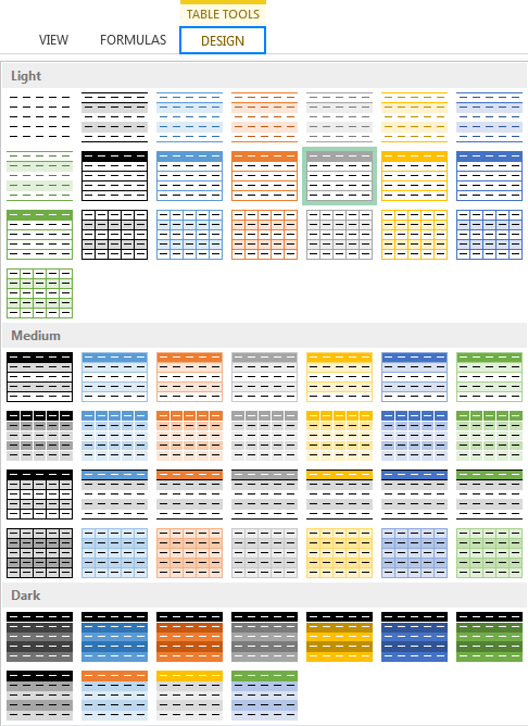
As you can see on the screenshot above, the Table Styles gallery provides a collection of 50+ inbuilt styles grouped into Light, Medium, and Dark categories.
You can think of an Excel table style as a formatting template that automatically applies certain formats to table rows and columns, headers and totals row.
Apart from table formatting, you can use the Table Style Options to format the following table elements:
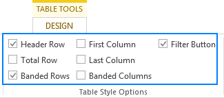
- Header row - display or hide the table headers.
- Total row - add the totals row at the end of the table with a list of functions for each total row cell.
- Banded rows and banded columns - alternate row or column shading, respectively.
- First column and last column - apply special formatting for the first and last column of the table.
- Filter button - display or hide the filter arrows in the header row.
The following screenshot demonstrates the default Table Style options:
How to choose a table style when creating a table
To create a table formatted with a specific style, do the following:
- Select the range of cells that you want to convert to a table.
- On the Home tab, in the Styles group, click Format as Table.

- In the Table Styles gallery, click the style that you want to apply. Done!
How to change table style in Excel
To apply a different style to an existing table, perform these steps:
- Click any cell within the table whose style you want to change.
- On the Design tab, in the Table Styles group, click the More button
 to show all available Excel Table styles.
 - Hover your mouse over the style you want to apply, and Excel will show you a life preview. To apply the new style, just click on it.
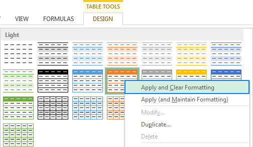
Tip. If you have applied any formatting to the table manually, e.g. highlighed certain cells in bold or with a different font color, selecting another Excel style will keep the manually applied formats in place. To apply a new style and remove any existing formatting, right-click on the style, and then click Apply and Clear Formatting.
How to change the default table style in Excel
To set a new default table style for a given workbook, right-click that style in the Table Styles gallery and select Set As Default:
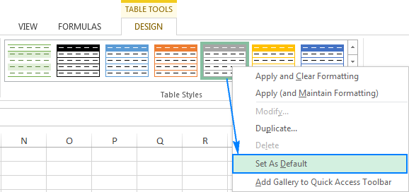
And now, whenever you click Table on the Insert tab or press the table shortcut Ctrl+T, a new table will be created with the selected default format.
How to create a custom table style
If you are not quite happy with any of the built-in Excel table styles, you can create your own table style in this way:
- On the Home tab, in the Styles group, click Format as Table. Or, select an existing table to display the Design tab, and click the More button
 .
. - Underneath the predefined styles, click New Table Style.
- In the New Table Style window, type a name for your custom table style in the Name box.
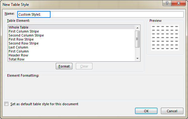
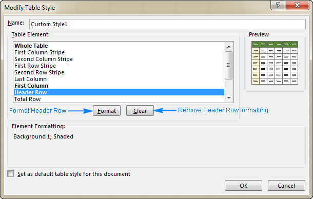
- Under Table Elements, select the element you want to format and click the Format button. The Format Cells dialog will open, and you select the desired formatting options on the Font, Border, and Fill tabs.
To remove existing formatting, click the element, and then click the Clear button.
Tips:
- The formatted table elements are highlighted in bold in the Table Element box.
- The formatting changes are shown in the Preview section on the right.
- To use the newly created table style as the default style in the current workbook, select the Set as default table quick style for this document box.
- Click OK to save your custom table style.
As soon as a custom style is created, it is automatically added to the Table Styles gallery:
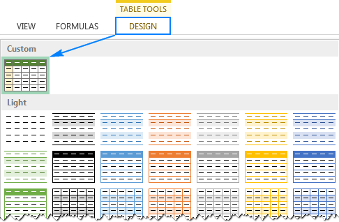
To modify a custom table style, go to the Table Styles gallery, right-click on the style, and click Modify…
To delete a custom table style, right-click on it, and select Delete.
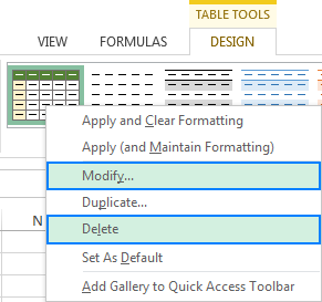
The built-in Excel table styles can neither be modified or deleted.
Tip. A custom table style is available only in the workbook where it is created. If you want to use it in another workbook, the fastest way is to copy the table with the custom style to that workbook. You can delete the copied table later and the custom style will remain in the Table Styles gallery.
How to apply a table style without creating an Excel table
If you want to quickly format the worksheet data with any of the inbuilt Excel table styles, but you don't want to convert a regular range to an Excel table, you can use the following workaround:
- Select a range of cells to which you'd like to apply a table style.
- On the Home tab, in the Styles group, click Format as Table, and then click the desired table style.
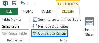
- Select any cell within a newly created table, go to the Design tab > Tools group, and click Convert to Range.
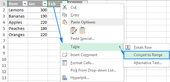
Or, right-click the table, point to Table, and click Convert to Range.
How to remove table formatting
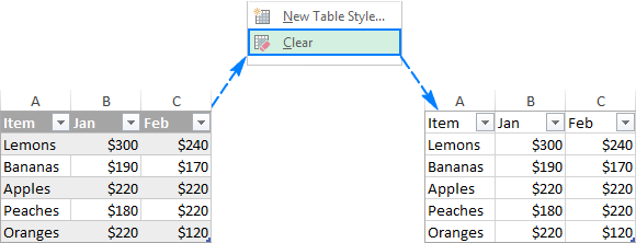
If you want to keep all features of an Excel table and remove only the formatting such as banded rows, shading and borders, you can clear the table format in this way:
- Select any cell in the table.
- On the Design tab, in the Table Styles group, click the More button.
- Underneath the table style templates, click Clear.
Tip. To remove a table but keep data and formatting, go to the Design tab Tools group, and click Convert to Range. Or, right-click anywhere within the table, and select Table > Convert to Range.
For more information on how to undo table format, please see How to remove table formatting in Excel.
That's how to manage table styles and formatting in Excel. I thank you for reading and hope to see you on our bog next week!
 by
by
55 comments
Hello Svetlana, appreciate all you do.
I can't figure out an easy-ish way to do "by-group" formatting in an Excel table.
Normal "green bar" pattern ... one colored row, one white row, repeat to end.
Desired pattern: alternating color by group ... when there are varying numbers of rows in each group.
E.g., a table of customer orders.
Order 1: 3 rows
Order 2: 13 rows
Order 3: 1 row
Order 4: 1 row
Order 5: 3 rows
I want automatic table formatting that visually color groups each order.
I can do it with non-table data with Conditional Formating, but I suspect that gets inefficient on a big table.
These steps for removing a table formatting do not work. There is no design tab, nor a clear button.
Hi! When you place the cursor on any cell in a table, your version of Excel may have a TABLE tab. Here you can apply table formatting. Table formatting differs between Excel versions.
how do i Apply a table style option to bold the item IDs in the first column of the table and contrast them with the other data.
Hi! You can change the formatting by condition using conditional formatting. There is no information to give you more precise advice.
What is the difference between the Table Styles option "Filter Button" in Excel and the Convert to Normal Range. Do they work the same. IF not, what is the difference.
Hi Michele,
The Filter button shows/hides the filter arrows in column headers. Please see Integrated sorting and filtering options.
The Convert to Range option changes a table back to a normal range and removes all features of a table such as automatic expansion, structured references, filter buttons, etc. For more information, please see How to convert an Excel table to a range.
Thank you very much, this helps me to remove the Formatting in a table.
yes, this blog helps me to get the solution
I'm having a problem with excels 09 Owners Solution 2. It will not let me format the cells a1:g73.
Help!
Hi!
Describe in detail what problem you have, and I will try to help you.
Hi, great instructions but missing one option. My cells already have formatting that I'd like to keep (e.g., fonts, color, filling, hyperlinks, etc).
I want to turn them into a table but keep the existing cell formatting, and just get the functionality of the table feature.
Can this be done?
Thanks!
Hello!
Create New table style. Go to Format as Table - New table style - Whole table. Then use this style when creating a new table. Previous formatting will not be changed
Hi Lisa,
Here's another way:
1. Convert your data into a table. The default table style will be applied messing up your formatting, but you ignore that for a moment.
2. On the Table Design tab, in the Table Styles group, select the very first style (None). Or, click the Clear button underneath the table styles.
That's it! The inbuilt formatting is gone, and your original one is preserved.
Sometimes excel offers the table styles as shown in the articles and sometimes it has different colors including pink and purple... why is that and how can I get it to always have purple as an option without creating my own format?
wtf!?! using clear as you specified deleted all of my table formats!!! thanks for nothing
Hello, I have been working in a pre-existing sheet with table formatting. I added about 10 additional columns (not in table format). Now I need to format them into the same table. Please advise - thank you in advance!
Hello Ben!
You need to resize the table. I recommend reading this article on our blog.
If you need any further assistance, please don’t hesitate to ask.
I have an excel which has hyperlinks from the other sheet of the same file. I have 20 to 30 sheets in one excel file, so when when I click the hyperlink, I usually have a hard time getting back to the main page which is the first sheet. Is there a way to have the main page sheet always appear like its being freeze so that even im on the 30th sheet I can still see the main sheet?
Hello
Can someone tell me how to take off a table once I have saved.
It is taking a very long time to open and close. I need it cleared back to the original info in my (large) spreadsheet without being in a table.
HELP! please :(
Thank you so much for this information. I couldn't find anything like this on YouTube, which is usually where I go. It would be great if you put this information on there for others. I needed to: Change an existing Table style that was formatted in Excel. I'm grateful!
Heather
I want to combine 100 excel workbooks(1st worksheet only) in one workbook(as a single worksheet) I also want to remove the first row from all workbooks but first. End result should be one sheet with a header row. Is this possible??
How to insert a .jpg file into an Excel
(Looking for a way to just insert the .jpg file into the cell, where it could be opened when needed, but otherwise, remain closed)
After adding a new row in the table, my auto row count function =SUBTOTAL(3,C$3:$C37) stops working properly in the first column. It messes up the new row count and the one previous to it.
It helped me, thank you!
Please solve my query:
I prepare a list of parked vehicles in the parking slot. On the daily basis how to check if a vehicle is parked continuously for more than one day?
Pl help.
You are the Best!
Svetlana Cheusheva you are so sweet....
When printing a table, is there a way to double space the rows (without inserting blank rows or increasing the row height)? Thanks.
how can i hide my formula in excel sheet .... nobody see the formula....
Hi Shanu,
You can hide your formulas by following these steps: How to hide formulas in Excel
hello!
Mam,
i want to know . how can i use index formula in multiple cell?
How types of data validation?
Hello...
I have two tables on same sheet (side by side) i.e. the rows of both the tables remains same. So when i filter the data of one table, the data on other near by table too changes which i don't expect it to do. Note that i don't want to place the tables one below another & want both tables on same sheet side by side.
Hope there will be solution to it.....
Thanks & Regards,
Merang
Just put one (small or hidden) column between the two tables
hi Svetlana Cheusheva
please can you tell me about how to delete pivottable in ms excel functional
thansk
Hello ! sir
In the Excel window, click anywhere inside the PivotTable report.
Under Pivot Table Tools, on the Options tab, in the Actions group, click Select, and then click Entire PivotTable.
Press the Delete key.
How may I convert a TXT file into excel WITHOUT creating the table or query format. I do not want it formatted as a table or a query, jsut a simple conversion to excel 2016. Or how can I remove the query and table formatting features once converted. It does not allow you to sort the entire page and the queriesa re not helpful if you do not need a table
Worked a charm! Thank you.
I am using a table format. When I add a line under the table i.e. the next row, it automatically extends the table along with all formats. Unfortunately the table has the date formatted to US instead of the UK (the rest of the logical world, in fact!). How can I change the format of the auto-generated rows? I can only seem to format the table from a visual perspective and now the cells themselves. At the moment I extend the table and then change the time format manually. Please advise,
Thanks.
*visual perspective but not the cells themselves.
Very helpful tips!!!
Hi!!
Whenever I import data from SQL server blue shaded table style if selected by default.
I need some other style. Even if I set it as default, still every time data is imported the blue shaded table comes to effect.
Please suggest.
Hi,
When the table comes from an external database (ie sql server in my case) , each update of the database turns off all my formattings.
How to disable this (the same we can do in a pivot table)
Hi,
I've been searching with no luck, if there is a way in which a custom table style o custom pivot table style can become the default style for every other workbook created after that.
Stefan:
Did you ever find an answer?
Hi
I have a question for you.
I have a database and the phone cell is write like this (623)700-4388 but I need get simple form like this 6237004388. Do you know if I can change this the list is big.. and I do not want to do this manually.
Hi Diego,
You can use Excel's Find and Replace command (Replace All), and replace the opening and closing parenthesis as well as the dash with nothing.
Or, you can do the same using the SUBSTITUTE function:
=SUBSTITUTE(SUBSTITUTE(SUBSTITUTE(A1,"(",""),")",""),"-","")
Hello Svetlana
Just want to say you are so smart!! I did not realize find&replace can actually do a lot of things!!!! Thank you for some idea, and hope I could apply that in future. :D
Hi Svetlana Cheusheva,
I have nearly 200 employees log in in log out details with different shift timing. Everyday the employee will come to the work at different shift, how to find out that the employee has come to the duty at correct time or not by using ms excel. We have 3 shifts. Morning to afternoon, afternoon to night and night to morning. For instance, today an employee called A came in the morning shift at 6 am and then tomorrow coming in the afternoon 2 pm and then the following day coming at night 10 pm..I wanna find out, whether he came to the shift to correct time or not and how many hours he worked. Can you give some idea in this regard?
Hello, just a thought, can you not give the poor employee a normal shift pattern? That might make it a lot easier for both of you!
Container Size
State 20 40
Sydney 520 730
How to pick value with two condition i-e
Sydney & 20 = 520 , Sydney & 40 = 430
Hello Asad,
You can use nested If's with embedded AND statements, like this:
=IF(AND(B1=20, A2="sydney"), 520, IF(AND(B1=40, A2="sydney"),430, ""))
If you are looking for something different, please clarify.
How To Insert If Condition On Time Format
Hello Aanand,
Sorry, it's impossible to advise anything based on such a generic description. Can you please elaborate on the task a bit more?