The tutorial shows 3 different techniques to plot a histogram in Excel - using the special Histogram tool of Analysis ToolPak, FREQUENCY or COUNTIFS function, and PivotChart.
While everyone knows how easy it is to create a chart in Excel, making a histogram usually raises a bunch of questions. In fact, in the recent versions of Excel, creating a histogram is a matter of minutes and can be done in a variety of ways - by using the special Histogram tool of the Analysis ToolPak, formulas or the old good PivotTable. Further on in this tutorial, you will find the detailed explanation of each method.
What is a histogram in Excel?
Wikipedia defines a histogram in the following way: "Histogram is a graphical representation of the distribution of numerical data." Absolutely true, and… totally unclear :) Well, let's think about histograms in another way.
Have you ever made a bar or column chart to represent some numerical data? I bet everyone has. A histogram is a specific use of a column chart where each column represents the frequency of elements in a certain range. In other words, a histogram graphically displays the number of elements within the consecutive non-overlapping intervals, or bins.
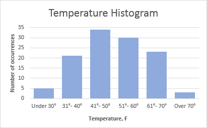
For example, you can make a histogram to display the number of days with a temperature between 61-65, 66-70, 71-75, etc. degrees, the number of sales with amounts between $100-$199, $200-$299, $300-$399, the number of students with test scores between 41-60, 61-80, 81-100, and so on.
The following screenshot gives an idea of how an Excel histogram can look like:
How to create a histogram in Excel using Analysis ToolPak
The Analysis ToolPak is a Microsoft Excel data analysis add-in, available in all modern versions of Excel beginning with Excel 2007. However, this add-in is not loaded automatically on Excel start, so you would need to load it first.
Load the Analysis ToolPak add-in
To add the Data Analysis add-in to your Excel, perform the following steps:
- In Excel 2010 - 365, click File > Options. In Excel 2007, click the Microsoft Office button, and then click Excel Options.
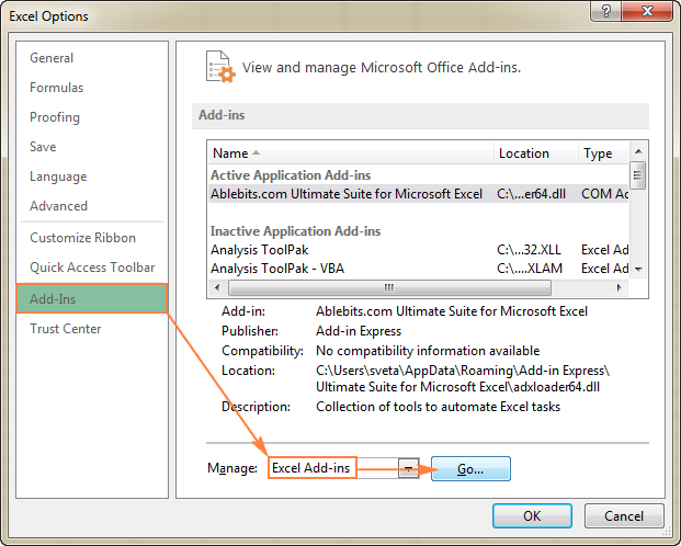
- In the Excel Options dialog, click Add-Ins on the left sidebar, select Excel Add-ins in the Manage box, and click the Go button.
- In the Add-Ins dialog box, check the Analysis ToolPak box, and click OK to close the dialog.
If Excel shows a message that the Analysis ToolPak is not currently installed on your computer, click Yes to install it.
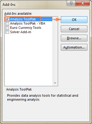
Now, the Analysis ToolPak is loaded in your Excel, and its command is available in the Analysis group on the Data tab.
Specify the Excel histogram bin range
Before creating a histogram chart, there is one more preparation to make - add the bins in a separate column.
Bins are numbers that represent the intervals into which you want to group the source data (input data). The intervals must be consecutive, non-overlapping and usually equal size.
Excel's Histogram tool includes the input data values in bins based on the following logic:
- A value is included in a certain bin if it is greater than the lowest bound and equal to or less than the greatest bound for that bin.
- If your input data contain any values greater than the highest bin, all such numbers will be included in the More category.
- If you do not specify the bin range, Excel will create a set of evenly distributed bins between the minimum and maximum values of your input data range.
Considering the above, type the bin numbers that you want to use in a separate column. The bins must be entered in ascending order, and your Excel histogram bin range should be limited to the input data range.
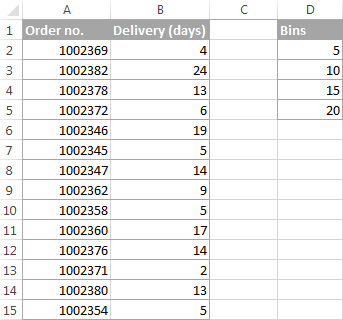
In this example, we have order numbers in column A and estimated delivery in column B. In our Excel histogram, we want to display the number of items delivered in 1-5 days, 6-10 days, 11-15 days, 16-20 days and over 20 days. So, in column D, we enter the bin range from 5 to 20 with an increment of 5 as shown in the below screenshot:
Make a histogram using Excel's Analysis ToolPak
With the Analysis ToolPak enabled and bins specified, perform the following steps to create a histogram in your Excel sheet:
- On the Data tab, in the Analysis group, click the Data Analysis button.

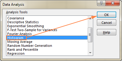
- In the Data Analysis dialog, select Histogram and click OK.
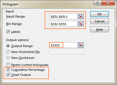
- In the Histogram dialog window, do the following:
- Specify the Input range and the Bin range.
To do this, you can place the cursor in the box, and then simply select the corresponding range on your worksheet using the mouse. Alternatively, you can click the Collapse Dialog button
 , select the range on the sheet, and then click the Collapse Dialog button again to return to the Histogram dialog box.
Tip. If you included column headers when selecting the input data and bin range, select the Labels check box.
- Select the Output options.
To place the histogram on the same sheet, click Output Range, and then enter the upper-left cell of the output table.
To paste the output table and histogram in a new sheet or a new workbook, select New Worksheet Ply or New Workbook, respectively.
Finally, choose any of the additional options:
- To present data in the output table in descending order of frequency, select the Pareto (sorted histogram) box.
- To include a cumulative percentage line in your Excel histogram chart, select the Cumulative Percentage box.
- To create an embedded histogram chart, select the Chart Output box.
For this example, I've configured the following options:
- Specify the Input range and the Bin range.
- And now, click OK, and review the output table and histogram graph:
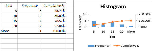
Tip. To improve the histogram, you can replace the default Bins and Frequency with more meaningful axis titles, customize the chart legend, etc. Also, you can use the design, layout, and format options of the Chart Tools to change the display of the histogram, for example remove gaps between columns. For more details, please see How to customize and improve Excel histogram.
As you've just seen, it's very easy to make a histogram in Excel using the Analysis ToolPak. However, this method has a significant limitation - the embedded histogram chart is static, meaning that you will need to create a new histogram every time the input data is changed.
To make an automatically updatable histogram, you can either use Excel functions or build a PivotTable as demonstrated below.
How to make a histogram in Excel using formulas
Another way to create a histogram in Excel is using the FREQUENCY or COUNTIFS function. The biggest advantage of this approach is that you won't have to re-do your histogram with each change in the input data. Like a normal Excel chart, your histogram will update automatically as soon as you edit, add new or delete existing input values.
To begin with, arrange your source data in one column (column B in this example), and enter the bin numbers in another column (column D), like in the screenshot below:
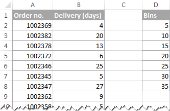
Now, we will use a Frequency or Countifs formula to calculate how many values fall into the specified ranges (bins), and then, we will draw a histogram based on that summary data.
Creating a histogram using Excel's FREQUENCY function
The most obvious function to create a histogram in Excel is the FREQUENCY function that returns the number of values that fall within specific ranges, ignoring text values and blank cells.
The FREQUENCY function has the following syntax:
- Data_array - a set of values for which you want to count frequencies.
- Bins_array - an array of bins for grouping the values.
In this example, the data_array is B2:B40, bin array is D2:D8, so we get the following formula:
=FREQUENCY(B2:B40,D2:D8)
Please keep in mind that FREQUENCY is a very specific function, so follow these rules to make it work right:
- An Excel Frequency formula should be entered as a multi-cell array formula. First, select a range of adjacent cells where you want to output the frequencies, then type the formula in the formula bar, and press Ctrl + Shift + Enter to complete it.
- It's recommended to enter one more Frequency formula than the number of bins. The extra cell is required to display the count of values above the highest bin. For the sake of clarity, you can label it "More" like in the following screenshot (but don't include that "More" cell in your bins_array!):
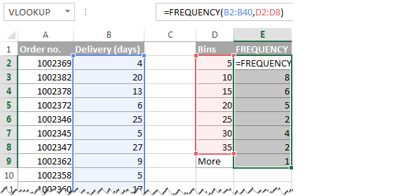
Like the Histogram option of the Analysis ToolPak, the Excel FREQUENCY function returns values that are greater than a previous bin and less than or equal to a given bin. The last Frequency formula (in cell E9) returns the number of values greater than the highest bin (i.e. the number of delivery days over 35).
To make things easier to understand, the following screenshot shows the bins (column D), corresponding intervals (column C), and computed frequencies (column E):
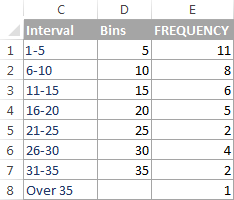
Note. Because Excel FREQUENCY is an array function, you cannot edit, move, add or delete the individual cells containing the formula. If you decide to change the number of bins, you will have to delete the existing formula first, then add or delete the bins, select a new range of cells, and re-enter the formula.
Making a histogram using COUNTIFS function
Another function that can help you calculate frequency distributions to plot histogram in Excel is COUNTIFS. And in this case, you will need to use 3 different formulas:
- The formula for the first cell - top bin (F2 in the screenshot below):
=COUNTIFS($B$2:$B$40,"<="&$D2)The formula counts how many values in column B are less than the smallest bin in cell D2, i.e. returns the number of items delivered within 1-5 days.
- The formula for the last cell - over the highest bin (F9 in the screenshot below):
=COUNTIFS($B$2:$B$100,">"&$D8)The formula counts how many values in column B are greater than the highest bin in D8.
- The formula for remaining bins (cells F3:F8 in the screenshot below):
=COUNTIFS($B$2:$B$40,">"&$D2,$B$2:$B$40,"<="&$D3)
The formula counts the number of values in column B that are greater than the bin in the above row and less than or equal to the bin in the same row.
As you see, the FREQUENCY and COUNTIFS functions return identical results:
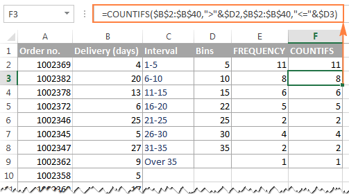
"What is the reason of using three different formulas instead of one?" you may ask me. Basically, you get rid of the multi-cell array formula and can add and delete bins easily.
Tip. If you plan to add more input data rows in the future, you can supply a bigger range in your FREQUENCY or COUNTIFS formulas, and you won't have to change your formulas as you add more rows. In this example, the source data are in cells B2:B40. But you can supply the range B2:B100 or even B2:B1000, just in case :) For example:
=FREQUENCY(B2:B1000,D2:D8)
Make a histogram based on the summary data
Now that you have a list of frequency distributions computed with either FREQUENCY or COUNTIFS function, create a usual bar chart - select the frequencies, switch to the Insert tab and click the 2-D Column chart in the Charts group:
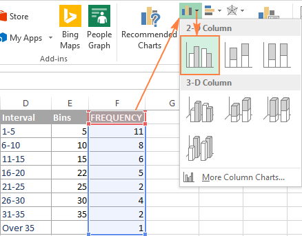
The bar graph will be immediately inserted in your sheet:
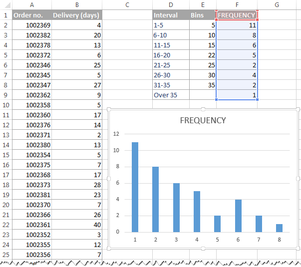
Generally speaking, you already have a histogram for your input data, though it definitely requires a few improvements. Most importantly, to make your Excel histogram easy to understand, you need to replace the default labels of the horizontal axis represented by serial numbers with your bin numbers or ranges.
The easiest way is to type the ranges in a column left to the column with the Frequency formula, select both columns - Ranges and Frequencies - and then create a bar chart. The ranges will be automatically used for the X axis labels, as shown in the below screenshot:
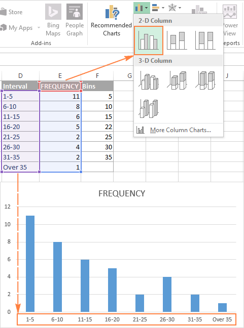
Tip. If Excel converts your intervals to dates (e.g. 1-5 can be automatically converted to 05-Jan), then type the intervals with a preceding apostrophe (') like '1-5. If you want the labels of your Excel histogram to display bin numbers, type them with preceding apostrophes too, e.g. '5, '10, etc. The apostrophe just converts numbers to text and is invisible in cells and on the histogram chart.
If there is no way you can type the desired histogram labels on your sheet, then you can enter them directly on the chart, independently of the worksheet data. The final part of this tutorial explains how to do this, and shows a couple of other improvements that can be made to your Excel histogram.
How to make a histogram with a PivotChart
As you may have noticed in the two previous examples, the most time-consuming part of creating a histogram in Excel is calculating the number of items within each bin. Once the source data has been grouped, an Excel histogram chart is fairly easy to draw.
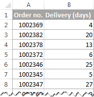
As you probably know, one of the fastest ways to automatically summarize data in Excel is a PivotTable. So, let's get to it and plot a histogram for the Delivery data (column B):
1. Create a pivot table
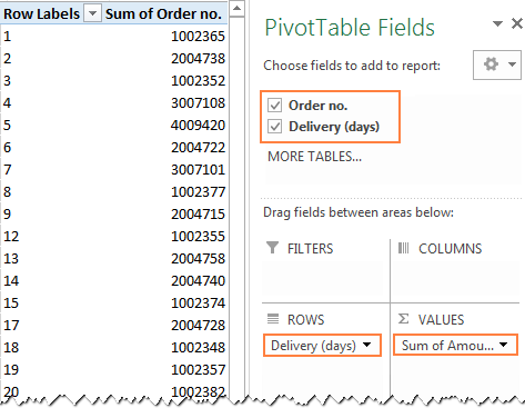
To create a pivot table, go to the Insert tab > Tables group, and click PivotTable. And then, move the Delivery field to the ROWS area, and the other field (Order no. in this example) to the VALUES area, as shown in the below screenshot.
If you have not dealt with Excel pivot tables yet, you may find this tutorial helpful: Excel PivotTable tutorial for beginners.
2. Summarize values by Count
By default, numeric fields in a PivotTable are summed, and so is our Order numbers column, which makes absolutely no sense :) Anyway, because for a histogram we need a count rather than sum, right-click any order number cell, and select Summarize Values By > Count.
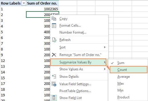
Now, your updated PivotTable should look like this:
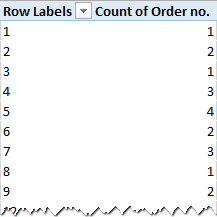
3. Create the intervals (bins)
The next step is to create the intervals, or bins. For this, we will be using the Grouping option. Right-click any cell under Row Labels in your pivot table, and select Group…
In the Grouping dialog box, specify the starting and ending values (usually Excel enters the minimum and maximum value automatically based on your data), and type the desired increment (interval length) in the By box.
In this example, the minimum delivery time is 1 day, maximum - 40 days, and the increment is set to 5 days:
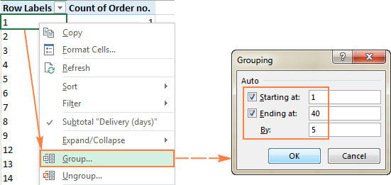
Click OK, and your pivot table will display the intervals as specified:
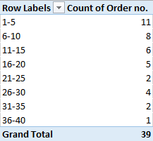
4. Plot a histogram
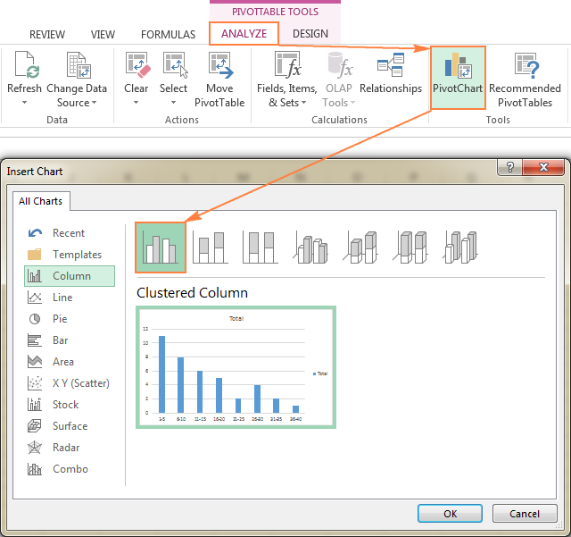
One final step is left - draw a histogram. To do this, simply create a column pivot chart by clicking the PivotChart on the Analyze tab in PivotTable Tools group:
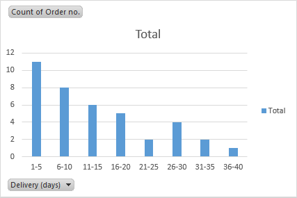
And the default column PivotChart will appear in your sheet straight away:
And now, polish up your histogram with a couple of finishing touches:
- Delete the legend by clicking the Chart Elements button
 and removing the tick from the Legend Or, select the legend on the histogram and press the Delete key on your keyboard.
 - Replace the default Total title with something more meaningful.
- Optionally, choose another chart style in the Chart Styles group on the PivotChart Tools > Design tab.
- Remove the chart buttons by clicking Field Buttons on the PivotChart Tools > Analyze tab, in the Show/Hide group:
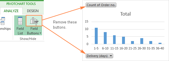
Additionally, you may want to achieve a conventional histogram look where bars touch each other. And you will find the detailed guidance on how to do this in the next and final part of this tutorial.
Customize and improve your Excel histogram
Whether you create a histogram using the Analysis ToolPak, Excel functions or a PivotChart, you might often want to customize the default chart to your liking. We have a special tutorial about Excel charts that explains how to modify the chart title, legend, axes titles, change the chart colors, layout and style. And here, we will discuss a couple of major customizations specific to an Excel histogram.
Change the axis labels on an Excel histogram chart
When creating a histogram in Excel with the Analysis ToolPak, Excel adds the horizontal axis labels based on the bin numbers that you specify. But what if, on your Excel histogram graph, you want to display ranges instead of bin numbers? For this, you'd need to change the horizontal axis labels by performing these steps:
- Right-click the category labels in the X axis, and click Select Data…
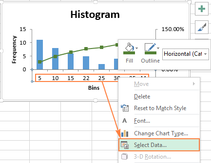
- On the right-hand side pane, under Horizontal (Category) Axis Labels, click the Edit button.
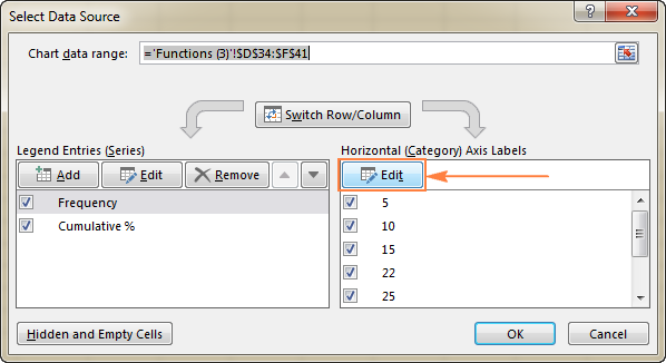
- In the Axis label range box, enter the labels you want to display, separated by commas. If you are entering the intervals, enclose them in double quotes like in the following screenshot:
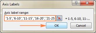
- Click OK. Done!
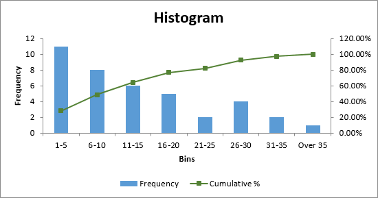
Remove spacing between bars
When making a histogram in Excel, people often expect adjacent columns to touch each other, without any gaps. This is an easy thing to fix. To eliminate empty space between the bars, just follow these steps:
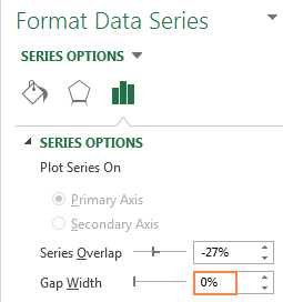
- Select the bars, right-click, and choose Format Data Series…
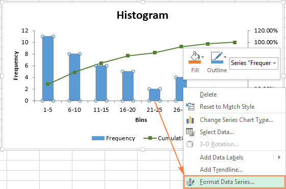
- On the Format Data Series pane, set the Gap Width to zero:
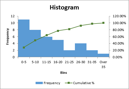
And voila, you have plotted an Excel histogram with bars touching each other:
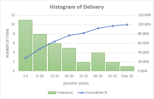
And then, you can embellish your Excel histogram further by modifying the chart title, axes titles, and changing the chart style or colors. For example, your final histogram may look something like this:
This is how you draw a histogram in Excel. For better understanding of the examples discussed in this tutorial, you can download the sample Excel Histogram sheet with source data and histogram charts. I thank you for reading and hope to see you on our blog next week.
 by
by
27 comments
Wow, I love this. Very easy and well explanatory. Great work.
Hi, Can anyone tell me if the Histogram function in Excel data analytics works for fractional data (e.g. 3.24, 5.22,,. etc.) or only with integer data (e.g. 324, 522...etc.)?
Thank you
This is an incredibly easy illustration love and fun to read. I am not any data analyst, used excell charts (graphs) and was assuming that histograms might be be a kind of it, when a close friend asked me to prepare a histogram of the data he provided. I instantly responded with a yes with my conventional charting ability. However to my surprise, histogram was something else that I now comprehend after reading this precious blog. Thanks.
this was super helpful thanks a lot.
Great work, keep it continue and easy to understand.thanks a lot!
Keep up the good work! Plain, concise and easy to follow English. Thanks a lot!
I'm grateful. Thanks for the Education
Under Excel 2010 under format data series - Series Options.I only see 2 iptions Where are the others?
Thanks for your detail explanation. I Want to clarify in Histogram chart,kindly to answer me..I am creating Row A1 to CZ151 data and the histogram chat...It won't take that huge amount of data..what is the Root cause..
Thanks for the perfect steps and clear diagrams! Got my histograms up and running.
Thanks for the help - needed to create a histogram in Excel 2010 and your instructions were right on the money
This is an excellent tutorial but I have to make a note from my experience. Up to version 2013 (and I suspect in later versions too), the FREQUENCY function and Data Analysis > Histogram produce the same results but these can actually be wrong in the case that the data used are results of calculations. That's because both methods use the binary representation of the numbers and this can cause those that are equal to a bin, to be included to the next range. For example, if the result of a calculation that you see in a cell e.g. B2, is 1.89 (no matter how many decimals you display), it is possible that the actual number used in making the histogram will be e.g. 1.890000000000000222044604925031 and you can see the difference between the two numbers with =B2-ROUND(B2,2)-0. If 1.89 is a bin, then the number should be included in the respective range but instead it is included in the next. One way to get around this is to round the results (e.g. =ROUND(B2,2)) before using them. Note also that simple coping and pasting as numbers has no effect. Another way is to use the functions COUNTIF, COUNTIFS or a pivot table instead which don't have this problem.
Thank you for the detailed explanation, it is really helpful!
Thank you for this post. This is very useful.
impressive summary i got something thanks
Thanks for this post. I found it easier to do the COUNTIFS version by using just COUNTIFS($H$3:$H$26,"<="&$B3) for all rows (cumulative histogram), then making another column where I calculated the histogram values as C3-C2, C4-C3, etc.
Impressive detail. I learned a lot.
Hi Team,
Kindly let me know why there is difference in frequency created by data analysis tool and frequency created by frequency formula. why it it is not same as data analysis tool
This women is great, I have read many articles of her and all of them are easily explained and detailed. Thanks for sharing your knowledge !!
Trying to customize a statistical histogram chart on one column of data. I want to set the range of the histogram bins, have the ticks labeled instead of the bins and want to set the left of the axis to zero. How do I do this customization?
Perfect explanation of histograms created from a frequency table that already exists. The only problem is that I want to create a polygon at the same time without having to insert a duplicate column of the frequency.
and if one is plotting it from column B against column D
please how can someone plot a histogram chart of one column against another column.
Thanks so much for making this step by step chart. I was trying to use a histogram on my entire dataset but the bins were all over the place. Your help makes it produce the graph as exactly what was needed. Thanks much!!
Thanks for giving such a good knowledge about 'Histogram' now i am looking for to present my work info. using Histogram..
Thanks so much! Very helpful during a last minute attempt to draw histograms for a dataset on Excel.