In this tutorial, you will learn how to create a number sequence in Excel with formulas. Additionally, we'll show you how to auto generate a series of Roman numbers and random integers - all by using a new dynamic array SEQUENCE function.
The times when you had to put numbers in sequence in Excel manually are long gone. In modern Excel, you can make a simple number series in a flash with the Auto Fill feature. If you have a more specific task in mind, then use the SEQUENCE function, which is specially designed for this purpose.
Excel SEQUENCE function
The SEQUENCE function in Excel is used to generate an array of sequential numbers such as 1, 2, 3, etc.
It is a new dynamic array function introduced in Microsoft Excel 365. The result is a dynamic array that spills into the specified number of rows and columns automatically.
The function has the following syntax:
Where:
Rows (optional) - the number of rows to fill.
Columns (optional) - the number of columns to fill. If omitted, defaults to 1 column.
Start (optional) - the starting number in the sequence. If omitted, defaults to 1.
Step (optional) - the increment for each subsequent value in the sequence. It can be positive or negative.
- If positive, subsequent values increase, creating an ascending sequence.
- If negative, subsequent values decrease, producing a descending sequence.
- If omitted, the step defaults to 1.
The SEQUENCE function is only supported in Excel for Microsoft 365, Excel 2021, and Excel for the web.
Basic formula to create a number sequence in Excel
If you are looking to populate a column of rows with sequential numbers starting at 1, you can use the Excel SEQUENCE function in its simplest form:
To put numbers in a column:
To place numbers in a row:
Where n is the number of elements in the sequence.
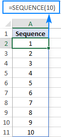
For example, to populate a column with 10 incremental numbers, type the below formula in the first cell (A2 in our case) and press the Enter key:
=SEQUENCE(10)
The results will spill in the other rows automatically.
To make a horizontal sequence, set the rows argument to 1 (or omit it) and define the number of columns, 8 in our case:
=SEQUENCE(1,8)

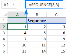
If you'd like to fill a range of cells with sequential numbers, then define both the rows and columns arguments. For instance, to populate 5 rows and 3 columns, you'd use this formula:
=SEQUENCE(5,3)
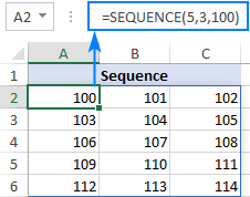
To start with a specific number, say 100, supply that number in the 3rd argument:
=SEQUENCE(5,3,100)
To generate a list of numbers with a specific increment step, define the step in the 4th argument, 10 in our case:
=SEQUENCE(5,3,100,10)
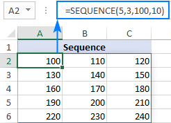
Translated into plain English, our complete formula reads as follows:

SEQUENCE function - things to remember
To efficiently do a sequence of numbers in Excel, please remember these 4 simple facts:
- The SEQUENCE function is only available with Microsoft 365 subscriptions and Excel 2021. In Excel 2019, Excel 2016 and earlier versions, it does not work since those versions do not support dynamic arrays.
- If the array of sequential numbers is the final result, Excel outputs all the numbers automatically in a so-called spill range. So, be sure you have enough empty cells down and to the right of the cell where you enter the formula, otherwise a #SPILL error will occur.
- The resulting array can be one-dimensional or two-dimensional, depending on how you configure the rows and columns arguments.
- Any optional argument that is not set defaults to 1.
How to create a number sequence in Excel - formula examples
Though the basic SEQUENCE formula does not look very exciting, when combined with other functions, it takes on a whole new level of usefulness.
Make a decreasing (descending) sequence in Excel
To generate a descending sequential series, such that each subsequent value is less than the preceding one, supply a negative number for the step argument.
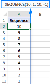
For example, to create a list of numbers starting at 10 and decreasing by 1, use this formula:
=SEQUENCE(10, 1, 10, -1)
Force a two-dimensional sequence to move vertically top to bottom
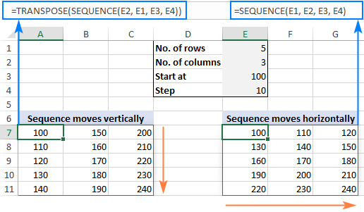
When populating a range of cells with sequential numbers, by default, the series always goes horizontally across the first row and then down to the next row, just like reading a book from left to right. To get it to propagate vertically, i.e. top to bottom across the first column and then right to the next column, nest SEQUENCE in the TRANSPOSE function. Please note that TRANSPOSE swaps rows and columns, so you should specify them in the reverse order:
For example, to fill 5 rows and 3 columns with sequential numbers starting at 100 and incremented by 10, the formula takes this form:
=TRANSPOSE(SEQUENCE(3, 5, 100, 10))
To better understand the approach, please have a look at the screenshot below. Here, we input all the parameters in separate cells (E1:E4) and create 2 sequences with the below formulas. Please pay attention rows and columns are supplied in different order!
Sequence that moves vertically top to bottom (row-wise):
=TRANSPOSE(SEQUENCE(E2, E1, E3, E4))
Regular sequence that moves horizontally left to right (column-wise):
=SEQUENCE(E1, E2, E3, E4)
Create a sequence of Roman numbers
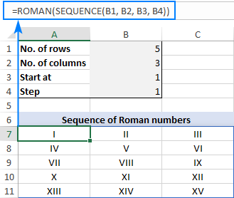
Need a Roman number sequence for some task, or just for fun? That's easy! Build a regular SEQUENCE formula and warp it in the ROMAN function. For example:
=ROMAN(SEQUENCE(B1, B2, B3, B4))
Where B1 is the number of rows, B2 is the number of columns, B3 is the start number and B4 is the step.
Generate an increasing or decreasing sequence of random numbers
As you probably know, in new Excel there is a special function for generating random numbers, RANDARRAY, which we discussed a few articles ago. This function can do a lot of useful things, but in our case it cannot help. To generate either an ascending or descending series of random whole numbers, we'll be needing the good old RANDBETWEEN function for the step argument of SEQUENCE.
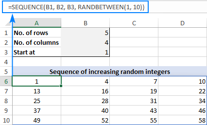
For example, to create a series of increasing random numbers that spills in as many rows and columns as specified in B1 and B2, respectively, and start at the integer in B3, the formula goes as follows:
=SEQUENCE(B1, B2, B3, RANDBETWEEN(1, 10))
Depending on whether you want a smaller or bigger step, supply a lower or higher number for the second argument of RANDBETWEEN.
To make a sequence of decreasing random numbers, the step should be negative, so you put the minus sign before the RANDBETWEEN function:
=SEQUENCE(B1, B2, B3, -RANDBETWEEN(1, 10))
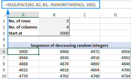
Note. Because the Excel RANDBETWEEN function is volatile, it will generate new random values with every change in your worksheet. As the result, your sequence of random numbers will be continuously changing. To prevent this from happening, you can use Excel's Paste Special > Values feature to replace formulas with values.
Excel SEQUENCE function missing
Like any other dynamic array function, SEQUENCE is only available in Excel for Microsoft 365 and Excel 2021 that support dynamic arrays. You won't find it in pre-dynamic Excel 2019, Excel 2016, and lower.
That's how to create sequence in Excel with formulas. I hope the examples were both useful and fun. Anyway, thank you for reading and hope to see you on our blog next week!
Practice workbook for download
Excel SEQUENCE formula examples (.xlsx file)
 by
by
399 comments
i need to create chart,
1 2 3 4 5
6 7 8 9 10
11 12 13 14 15
16 17 18 19 20
leave a blank and then generate
21 22 23 24 25
26 27 28 29 30
31 32 33 34 35
36 37 38 39 40
blank cell
41 42 43 44 45
46 47 48 49 50
51 52 53 54 55
56 57 58 59 60
suggest pls
Hello,
I have a question regarding the "n" in the SEQUENCE Function.
Can it be unknown?
From a table, I would like the formula to list all the data that are above 13%. I can do this using the INDEX, SORT and FILTER functions. But I do not know how many people will be above 13%. Is there a solution to this?
My formula is as per the below:
=INDEX(SORT(FILTER(Master!F4:AC248,Master!AC4:AC248>=13%),24,-1),SEQUENCE(20),{1,24})
Thanks,
Matt
Hello!
In the SEQUENCE function, specify the maximum number of values (for example, 245). To ignore errors, use the IFERROR function.
=IFERROR(INDEX(SORT(FILTER(Master!F4:AC248,Master!AC4:AC248>=13%),24,-1),SEQUENCE(245),{1,24}),"")
Hope this is what you need.
Hi Alexander,
Thank you for taking the time to reply and apologies for the delay of my answer.
Unfortunately this does not work for me so had to change the formula to the below:
=INDEX(SORT(FILTER(Master!B4:AC243,(Master!S4:S243="GBP")*(Master!M4:M243=""),"No results"),28,-1),SEQUENCE(20),{5,28})
So what this does is giving me the 20 top percentages. But only 8 of them are above 13%.
How can I make sure that with this formula, it removes the percentages that are under 13%?
(if this is possible).
Thanks,
Matt
Hi!
Without seeing your data it is difficult to give you any advice.
If you are fetching data from column AC, add a filter condition to the formula:
FILTER(Master!B4:AC243,(Master!S4:S243=”GBP”)*(Master!M4:M243=””)*(Master!AC4:AC243>13%),”No results”)
I hope I answered your question.
Hi Alexander,
Works a treat! Thank you so much!
Matt
I want to enter the following in the column , so kindly help me out:
A1 : 0-1
A2 : 1-2
A3 : 2-3
and so on.
whereas A1, A2, A3 are the address of the Column and the numerics are the value to be entered.
Hello
I would like to have this numbering sequence:
01-G
02-G
03-G
Thanks in advance for the help
Hello!
You can use this formula:
=TEXT(SEQUENCE(10,1,1,1),"00")&"-G"
Add text to the sequence of numbers using the & operator.
Hi Sir,
I would like to make following sequence, which would be changing based on names in other column. The number of rows with the same name is random - sometimes 5 rows, sometimes 1 row:
2021-1000 John
2021-1000 John
2021-1000 John
2021-1001 Tim
2021-1001 Tim
2021-1001 Tim
2021-1002 James
2021-1002 James
2021-1003 Michael
I would appreciate your help.
Hi!
What you want to do is not sequence. This is a random number of duplicates. I'm really sorry, looks like this is not possible with the standard Excel options.
Hello, I am trying to make a SEQUENCE based on the text in the cell next to it.
Column B can be either IC, IG, IB, or any other 2 letter
Column C is a number list 21001 21002 21003 and so on.
However the number can repeat based on the letters in Column B. So I need the sequence to be based on the next available number that relates to the letters in column B.
I hope that make sense
Hello!
To make a sequence of numbers with a condition, use the formula
=21000+COUNTIF($B$2:B2,B2)
Hope I understood the problem correctly.
It did work thank you. Now if I can get my co workers to stop skipping number
Hello I had a follow up on this. I changed the formula a little to exclude texts from the count so it looks like this now.
=21000+COUNTIFS('2022'!$D$3:D3,D3,'2022'!$K$3:K3,"CO",'2022'!$K$3:K3,"NCCO")+1
My problem is when I go to the next cell the is jumps numbers equal to how many cells are used
EX.
=21000+COUNTIFS('2022'!$D$3:D5,D4,'2022'!$K$3:K5,"CO",'2022'!$K$3:K5,"NCCO")+1
=21000+COUNTIFS('2022'!$D$3:D7,D5,'2022'!$K$3:K7,"CO",'2022'!$K$3:K7,"NCCO")+1
=21000+COUNTIFS('2022'!$D$3:D9,D6,'2022'!$K$3:K9,"CO",'2022'!$K$3:K9,"NCCO")+1
^ ^ ^
I put arrows where the numbers jump. Why would it do that and not follow the order? I can not seem to stop this.
I am constantly having to create numbering sequences that look like this:
100 000001
100 000002
three numbers, space and then 6 numbers with only the last 6 numbers increasing. What would be the formula to achieve that?
Thanks
Hi!
You can use a custom number format to repeat zeros.
Use the TEXT function to display a number in this custom format.
="100 " & TEXT(SEQUENCE(100,,1,1),"*00000##")
Hope this is what you need.
I am in need of a way to have a number increase by one each day for a production report. Example
4 departments in separate columns. Above each heading is the number of days worked. Is there a way increase those days by 1 automatically each day?
Thanks in advance!
Is there a way to sequence numbers if the numbers look like this------
PI-2021-07-0480
PI-2021-07-0481
Please advise -
Dawn
Hi,
what if I have number series like
[1,2,3,4,5], [11,12,13,14,15], [21,22,23,24,25] and so on in one column until some hundred,
is there any way to do this?
thank you!
Good Day
We would like to have the following data on a separate line for a raffle draw. They unfortunately did the numbering as :
31100-31127
32656-32697
34729-34750
90784-90828
92159-92198
333-336
851-856
116-119
867-858
859
2070-2079
2709-2713
2569-2573
337-340
341-343
860
861-861
Is there a way to have them in one column in order?
Hi!
I'm really sorry, we cannot help you with this.
Hello,
I suggest a helper column in column B with this formula (and copy down):
=IF(ISNUMBER(A1),A1,VALUE(LEFT(A1,FIND("-",A1)-1)))
Then in cell C1, have a sort formula =SORT(A1:B1000,2)
Hope this solves the problem.
André
Hello sir, how about sequence with text in rows, like:
var 1 var 2 var 3
And so on.
Thank you for your help
Hello!
Please re-check the article above since it covers your task. The SEQUENCE function works on a row as well.
I've tried
="var "&SEQUENCE(1,50,1,1)
But it doesn't work
Hi!
It works for me. What doesn't work for you? SEQUENCE function available in Microsoft Excel 365.
how about
KD1-20
KD21-40
KD41-60
and so on.
tnx
Hi!
Try the following formula:
="KD"&CEILING(SEQUENCE(100,1,1,20)/1,1)&"-"&CEILING(SEQUENCE(100,1,1,20)/1,1)+19
i forgot something formula for
1kd 1 - 20
2kd 21 - 40
3kd 41 - 60
4kd 61 - 80
thank u sir godbless
Hello Sr
how can I do a sequence of rows every 8 repetitive number, every 8 rows same number, then the next one 8 times, etc. Example: the patern is same number 8 rows or 8 times, then next number ther 8 rows or times:
1
1
1
1
1
1
1
1
2
2
2
2
2
2
2
2
3
3
3
3
3
3
3
3
thank you
Hello!
Please use the following formula
=CEILING(SEQUENCE(800,1,1,1)/8,1)
thank you
Thanks
I am currently stuck on a problem while creating an MLB pitching model. I would like to distribute the number of batters faced across the 9 positions in a batting order. Lets say a pitcher faces 23 batters during his out outing I would like to distribute that across the 9 batting order spots in sequential order. In doing this manually I know the pitcher would face the first 5 batters 3 times and the 6-9th batter 2 times. How can I create a running tally that distributes those 23 batters across the 9 batting order spots -- more simply put how can I tally the number 23 across 9 cells in sequential order? Thank you in advance if you can solve this riddle!
I want to generate the following pattern in excel cells. Would it be possible
0000000000
1000000000
1100000000
1110000000
1111000000
....
I want to generate this kind of number but I am having difficulty. Anyone can help me?
=VLOOKUP(G2,O2:P23,2,FALSE)
=VLOOKUP(G3,O2:P23,2,FALSE)
=VLOOKUP(G4,O2:P23,2,FALSE)
=VLOOKUP(G5,O2:P23,2,FALSE)
=VLOOKUP(G6,O2:P23,2,FALSE)
=VLOOKUP(G7,O2:P23,2,FALSE)
=VLOOKUP(G8,O2:P23,2,FALSE)
=VLOOKUP(G9,O2:P23,2,FALSE)
=VLOOKUP(G10,O2:P23,2,FALSE)
The G Is the one only rising. Thank you to anyone who can help.
Hi!
When you copy the formula down the column, G2 will change to G3, G4, and so on.
Hi,
1 have 5 digits number, for example 01234, from that number I want to generate 2 digits number for all the possible sequence, so 00, 01, 02, 03, 04, 10, 11, 12, 13, 14, 20, 21,... and so forth.
Any way to do this? TYIA
would it be possible to sequence numbers but end on the number that is in the next column.
example:
1 6
2 6
3 6
4 6
5 6
6 6
1 3
2 3
3 3
1 5
2 5
We are using the info for a data merge for bundles. so the outcome would be "Bundle 1 of 6"
Thank you
Hello!
You have not written what is the source data. I am assuming column B. Perhaps this formula will work -
=COUNTIF($B$1:B1,B1)
After that you can copy this formula down along the column.
If this is not what you wanted, please describe the problem in more detail.
Sorry, Can you tell I don't know what I'm doing?
I was able to plug this in and worked. But I do see when I scroll down and some of the "bundles" are combined together and then go back to correct sequence. what could cause this?
example: Source is column B.
1 8
2 8
3 8
4 8
5 8
6 8
7 8
8 8
8 7
9 7
10 7
11 7
12 7
13 7
14 7
1 9
2 9
3 9...
Hello!
What formula are you using?
The formula used was =COUNTIF($B$1:B1,B1)
After some testing I realized that the repeating bundles would start from the previous similar bundles. see below.
example:
1 5
2 5
3 5
4 5
5 5
1 7
2 7
3 7
4 7
5 7
6 7
7 7
6 5
7 5
8 5
9 5
10 5
What if we want this
1 6 11
2 7 12
3 8 13
4 9 14
5 10 15
Sequence reference for Bookmark pdf
1st row is 1 - 5 (sequence)
2nd row is 2 - 2
3rd row is 2 - 4
4th row is 4 - 5
5th row is 6 - 7 (sequence)
6th row is 8 - 9 (sequence)
7th row is 9 - 11
8th row is 10 - 11 (sequence)
9th row is 14 - 15 (sequence)
How to check missing sequence 12 - 13
For above type of page range.
Hello,
I am trying to have a One Column, with the following parameters:
First 20 Columns (1-20) is 1
Next 30 Column (21-50) is 2
Next 40 Column (51-90) is 3 and so forth.
Also I want to make it dynamic where I can change the columns i.e Instead of having the first 20 columns to 1, I can plug into a cell 30 and the first 30 column is 1 and the rest adjust accordingly.
I am create a training plan and I can decide to have the first 20 go to training in Wave 1 or first 30 to Wave 2 etc.
Please how can I create this formula.
Thanks for your help.
Oluseyi
This is perfect - Thank You!
how can I generate this kind of Sequence
Chapter: 1 - 3
Chapter: 4 - 6
Chapter: 7 - 9
.
.
.
.
Hello,
What would the formula be to create this sequence?
A1001A A1001B A1001C A1001D A1002A A1002B A1002C A1002D A1003A A1003B A1003C A1003D
A1004A A1004B A1004C A1004D A1005A A1005B A1005C A1005D A1006A A1006B A1006C A1006D
Where the last letter in the series ends with "D", but the preceding number will increase as the sequence proceeds.
Thanks
Hello!
If I understand your task correctly, the following formula should work for you:
="A"&(1000+CEILING(SEQUENCE(1000,1,1,1)/4,1)) & CHOOSE(TRUNC(MOD((ROW(A1:A1000)-1)/1,4)+1),"A","B","C","D")
Hope this is what you need.
I really prefer the sequence function. However, my computer, Microsoft 2016, doesn't exist the function. I accessed to the internet and i found that Sequence Function can be only supported by Microsoft 360. How can i install the function and does it affect my computer if i install it? Thank you very much
Hi thank you so much for your informative guidance.
This is pdf index page sequence.
1-4
5-88
(37-38
60-61
61-63
64-65
64-64)
89-101
(91-92
94-95)
103-108
107-108
How to check missing sequence 102...
eg. sequence of numbers 1-1, 2-2, 4-5. Number 3 was skipped..
I have 4 sheets , the number of rows is random for each sheet. How to make the sequential number continue from sheet 1 to sheet 4 meanwhile the number of rows is random .
Hello!
Find the maximum number on the previous sheet using the MAX function and add 1 to it.
=MAX(Sheet2!A:A)+1
Then, on the current sheet, simply add 1 to this number.
Hello,
I hope you can help. I am trying to identify the number of transactions per date and per supplier, and create a sequence from this.
For example, on 20th May 2021, 1 transaction was from British Gas, 3 transactions were put through from Amazon, and 1 from Sainsbury's. I assume a formula can cluster per unique supplier whilst incrementing sequentially, I just haven't cracked it yet:
20210520-01
20210520-02
20210520-02
20210520-02
20210520-03
Essentially, I want to match 3 transactions to one from a Cash Book to a Bank Statement. The CB would list 3 individual items from Amazon and the Bank would show one transaction. I would like to be able to cross-reference automatically/dynamically. That way I can SUMIF and MATCH to reconcile (hopefully).
If there is a better way, please say! Currently, I am working on historic 'chunks' of formula and concatenating. I thought it was time to get up to date.
Also, I can only get the date sequence as 44336 when appearing in a formula. That's fine if it has to be this way, I'd just prefer it to be Gregorian if possible. Do you know if I can use a format for this?
Much appreciated in anticipation.
Hello!
I’m sorry but your task is not entirely clear to me.
You can apply a standard or custom date format to the 44336 as described in this guide.
I want sequence something like this:
1
2
1
2
1
2
1
2
.
.
.
.
.
etc.
how to achieve this?
Hi!
A sequence is a series of consecutive numbers: 1,2,3 ... or 3,5,7 ... Each next number is not less than the previous one.
Your example is not a sequence. Write 1 and 2 in the cells and copy them down the column.
Hello,
I have a sequence generated say in one column on one sheet (List A)
Now I want to assign the numbers from this list A at various place on different sheet. Is there a way to every time assign number from this list A which is not already assigned (taken up earlier)
- For now I have created a named list B combining all ranges in which I have assigned (manually) the number from from this list A.
- Then in next column to list A put in a look up for each sequence number from this named list B to indicate which one is used up and which one not using 1 an 0. lets say this is indicator column
- Further in one cell on sheet where i assign the numbers, put a formula to look up in this indicator column to find the first 0 and correspondingly return the sequence number against it. thus displaying the next number available for assignment.
- I then manually assign (type) that displayed number from above cell and since that cell where i type the number is in the range included in list B, the cell displaying the next sequence updates to next one and so on continues.
Is it possible to automatically do this instead of me typing it manually. If we can identify the formula then it would be great.
i want a sequence where number is skipped
eg. sequence of days where sunday is skipped
1
2
3
4
5
6
8
9
10
11
12
13
15 ......
Hello!
The formula below will do the trick for you:
=SEQUENCE(300,1,1,1)+CEILING(SEQUENCE(300,1,1,1)/6,1)-1
Hope this is what you need.
Greetings.
I want to make sequence like these:
15x number 1
53x number 2
45x number 3
...
How can I do this?
Than you in advance
Hi,
Sorry, it's not quite clear what you are trying to achieve. What is the pattern in your numbers?
DEAR SIR
I want to make sequence in different cells i mean selected cells .
make select cells and put sequence in selected cell .
not upcoming cell.
Hi!
An Excel formula can only work over a continuous range. It is not possible to select individual cells.
I have a sequence of numbers, let's say:
1
3
4
20
22
and would like Excel to return on a cell(another sheet) the next available number in the given column, starting in 1 to n, if this makes sense.
Is this possible?
Thanks
Hello!
Write down your numbers starting at cell A2. Write this formula in cell B2
=MIN(FILTER(SEQUENCE(100,1,1,1),(SEQUENCE(100,1,1,1)>A2)*(SEQUENCE(100,1,1,1)<>A3)*(SEQUENCE(100,1,1,1)<>B1)))
and then copy it down along the column.
You can learn more about FILTER function in Excel in this article on our blog.
Hope this is what you need.
i have a sequence of number
AAA0001 --- AAA9999 , after the 9999 the next number i need is AAB0001 and continue increasement .
please help , and the alphabet increase is without "I" and "o" .
thanks !
Hi,
I'm really sorry, we cannot help you with this task. Your task cannot be accomplished with Excel formulas.
I'm spending way too much time on this but who doesn't like a good excel challenge.
after playing with the start value I was able to make it a bit more elegant
this solves the no i and o in the letter sequence and skips from 9999 to 0001
also you can change the number series from 9999 to 999 in P2
you can drag the top cell across to continue the series in the next column as this series exceeds the max rows allowed in a column.
=CHAR(65 + MOD(SEQUENCE(1048576,1,(COLUMN()-1)*1048576,1)/(24^2*$P$2),24) + IFS(MOD(SEQUENCE(1048576,1,(COLUMN()-1)*1048576,1)/(24^2*$P$2),24)>12,2,MOD(SEQUENCE(1048576,1,(COLUMN()-1)*1048576,1)/(24^2*$P$2),24)>7,1,TRUE,0)) & CHAR(65 + MOD(SEQUENCE(1048576,1,(COLUMN()-1)*1048576,1)/(24*$P$2),24) + IFS(MOD(SEQUENCE(1048576,1,(COLUMN()-1)*1048576,1)/(24*$P$2),24)>12,2,MOD(SEQUENCE(1048576,1,(COLUMN()-1)*1048576,1)/(24*$P$2),24)>7,1,TRUE,0)) & CHAR(65 + MOD(SEQUENCE(1048576,1,(COLUMN()-1)*1048576,1)/($P$2),24) + IFS(MOD(SEQUENCE(1048576,1,(COLUMN()-1)*1048576,1)/($P$2),24)>12,2,MOD(SEQUENCE(1048576,1,(COLUMN()-1)*1048576,1)/($P$2),24)>7,1,TRUE,0)) & RIGHT("00000" & MOD(SEQUENCE(1048576,1,(COLUMN()-1)*1048576,1),($P$2))+1,LEN($P$2))
ok I have refined my previous answer a little
set $C$2 to either 999 or 9999 depending on the number series you want
then use this formula to get the series you asked for.
No letters i or o and skip from 9999 to 0001
This was a fun puzzle!!!
=IF(SEQUENCE(1048576)>$C$2*24^2,"B","A") & CHAR(65 + INT(MOD(SEQUENCE(1048576)/(24*$C$2)- 0.000001,24)) + IFS(INT(MOD(SEQUENCE(1048576)/(24*$C$2)- 0.000001,24))>12,2,INT(MOD(SEQUENCE(1048576)/(24*$C$2)- 0.000001,24))>7,1,TRUE,0)) & CHAR(65 + INT(MOD(SEQUENCE(1048576)/($C$2)- 0.000001,24)) + IFS(INT(MOD(SEQUENCE(1048576)/($C$2)- 0.000001,24))>12,2,INT(MOD(SEQUENCE(1048576)/($C$2)-0.000001,24))>7,1,TRUE,0)) & RIGHT("00000" & ROUNDUP(MOD(SEQUENCE(1048576),($C$2)+0.000001),0),LEN(C2))
for even more fun ;o)
you can use this formula and drag from a1 to k1 or more
This will continue the series since column limit in excel doesn't go far enough for your series
in this case the number series 999 or 9999 is in $M$2
=CHAR(65 + INT(MOD((SEQUENCE(1048576)+((COLUMN()-1)*1048576))/(24^2*$M$2)- 0.0000001,24)) + IFS(INT(MOD((SEQUENCE(1048576)+((COLUMN()-1)*1048576))/(24^2*$M$2)- 0.0000001,24))>12,2,INT(MOD((SEQUENCE(1048576)+((COLUMN()-1)*1048576))/(24^2*$M$2)- 0.0000001,24))>7,1,TRUE,0)) & CHAR(65 + INT(MOD((SEQUENCE(1048576)+((COLUMN()-1)*1048576))/(24*$M$2)- 0.0000001,24)) + IFS(INT(MOD((SEQUENCE(1048576)+((COLUMN()-1)*1048576))/(24*$M$2)- 0.000001,24))>12,2,INT(MOD((SEQUENCE(1048576)+((COLUMN()-1)*1048576))/(24*$M$2)- 0.000001,24))>7,1,TRUE,0)) & CHAR(65 + INT(MOD((SEQUENCE(1048576)+((COLUMN()-1)*1048576))/($M$2)- 0.000001,24)) + IFS(INT(MOD((SEQUENCE(1048576)+((COLUMN()-1)*1048576))/($M$2)- 0.000001,24))>12,2,INT(MOD((SEQUENCE(1048576)+((COLUMN()-1)*1048576))/($M$2)-0.000001,24))>7,1,TRUE,0)) & RIGHT("00000" & ROUNDUP(MOD((SEQUENCE(1048576)+((COLUMN()-1)*1048576)),($M$2)+0.000001),0),LEN($M$2))
Hello,
I have a sequence of numbers, let's say:
1
3
4
20
22
and would like Excel to return on a cell(another sheet) the next available number in the given column, starting in 1 to n, if this makes sense.
Is this possible?
Thanks
Hi, thank you, Sir Alexander, I'm working on making a sequence of Admission number like
1910404001
19104040002
1910404003
,,,,
,,,,,
,,,
Please help me, thank you?
Hi,
The constant 1910404 can be combined with a changing value using the & operator. To always have 3 digits in a number, use the TEXT function.
I’ll try to guess and offer you the following formula:
=1910404&TEXT(SEQUENCE(100,1,1,1),"000")
How can i make sequence of number series with one column or row blank.
1 2 3 4 5 6
- - - - - -
7 8 9 10 11
- - - - - -
Hi,
You can use the formula
=SEQUENCE(1,10,1,1)
Hi, I am looking to take data from one column and create a sequential number in another column. However the data in my reference column (location codes) are duplicated in more than one row but I need my sequential number column to be the same value for each location code. Example: My first entry is Location code K051 that has three rows of data so it's sequential number should be 1 for each of the three rows. Next location code is K052 that has five rows of data so it's sequential number column should be 2 for each of it's 5 rows.
Each location code could have a varying amount of rows associated.
Is there a formula that can create these sequential numbers? Thank you!
Hello!
If the Location code is written in column A, the order number of each code can be obtained using the formula
=MATCH(A2,UNIQUE($A$2:$A$20),1)
After that you can copy this formula down along the column.
i want to make a series of 3 digit 'n' numbers
please help
Hi,
You can get 3-digit numbers with this formula:
=SEQUENCE(900,1,100,1)
If this is not what you wanted, please describe the problem in more detail.
Hi,
I'm trying to generate a sequence of numbers in the below order. Could you please help?
40000 / 01
40002 / 03
40004 / 05
40006 / 07
40008 / 09
...
...
...
etc
Hello!
The formula below to solve your task:
=40000+(ROW(A1)-1)*2&" / "&TEXT(ROW(A1)*2-1,"00")
Hi Alex,
Highly appreciate your quick response. Excel shows that 'there's a problem with this formula'.
Thanks again!!!
Thomas
I'm wondering if anyone could help me.
I am trying to generate some 1-column sequences like this:
1001-01
1001-02
1001-03
1002-01
1002-02
1002-03
1003-01
1003-02
1003-03
1004-01
(etc.)
Hello!
If I understand your task correctly, the following formula should work for you:
=CEILING(ROW(A3001)/3,1)&" - 0"&TRUNC(MOD((ROW(A1)-1)/1,3)+1)
I hope my advice will help you solve your task.
this works great but how do I use a dynamic function with the solution?
I have 2 numbers set by the user: a1 = 15 and b1 = 3
from these two inputs I would like to dynamically create a sequence that goes:
1.1
1.2
1.3
2.1
2.2
.... until 15.3
is this possible?
after playing around with John's "puzzle" below I came up with this to solve my own issue:
=INT(MOD(SEQUENCE($A$1*$B$1,1,0,1)/$B$1,$A$1)) + 1 & "." & MOD(SEQUENCE($A$1*$B$1,1,0,1),$B$1) + 1
somehow doing it with letters from the AAA0001 loop helped me figure out my own loop better.
Hi!
Replace A3001 with A1 in the formula above.
yes but that is not making use of the dynamic array function
Thank you for your reply. I understood how that worked but the ideal solution for me is one that uses a dynamic array. not a drag down approach.
Hello!
Instead of the ROW function, use SEQUENCE:
=CEILING(SEQUENCE(45,1,1,1)/3,1)&"."&TRUNC(MOD((SEQUENCE(45,1,1,1)-1)/1,3)+1)
Hope this is what you need.
I am wondering if you can make a sequence where the number changing is not the last character? I want it to be like this, with the stars included? I need it to go from 1-99. Thanks for the help!!
*R1-01-01-01*
*R1-01-01-02*
*R1-01-01-03*
*R1-01-01-04*
*R1-01-01-05*
Hi!
If I got you right, the formula below will help you with your task:
="*R1-01-01-"&TEXT(SEQUENCE(99,1,1,1),"00")&"*"
Hope this is what you need.
Hello
Sir I want generate the series of mobile phone numbers like 2301230000 to 2301239999 I don't know how I can?
Hello Farhan,
You can use a formula like this:
=SEQUENCE(9999,1,2301230000)
Where 9999 is how many numbers you want to generate.
Hi thank you so much for your informative guidance.
I have a question. How would the sequence function work in case I wanted to repeat the same number twice?
e.g.
2175
2175
2176
2176
2177
2177
2178
2178
etc.
Thanks appreciate your help!
Hello!
Use the following formula/the formula below to solve your task:
=CEILING(ROW(A4349)/2,1)
After that you can copy this formula down along the column.
Sir, how to make a formula for consecutive numbers but different from dates
Example
01 jan 2021 02 jan 2021
1028365-628 1034664-629
Thanks
Hi!
Your question is not entirely clear, please specify.
how to combine the formula ARRAY_CONSTRAIN(ARRAYFORMULA(SEQUENCE(1,5,628,1)), 1, 5) with CONVERT
I want a generate a sequence of numbers in order from 1 to 25. But have them starting again from 1 after 25. How would I modify this formula to satisfy this.
I have the same , I need to have a sequence number generated automatically and continuance from page one to the next page ... I need to use this sequence as an order number so every time I place an order I have to get an automatic number ... is it possible ?
thank you & appreciate
Hello!
For automatic line numbering from 1 to 25, use the formula
=TRUNC(MOD((ROW(A1)-1),25)+1)
After that you can copy this formula down along the column.
so if I need to make my number start from 10001 :
how it should look like
Interesting piece! I am creating a spreadsheet for my wife who is a potter. All pieces, let's say 'started', are listed in the spreadsheet starting 1 and obviously going down the sheet 2,3,4 etc. However, owing to the nature of her activity, not all pieces get to the point of being saleable items - thus, the final product codes for the saleable items are also consecutive, but there might be gaps between rows, where certain pieces are rejected i.e. product code 0001,0002, gap, gap, gap, 0003 etc. Is it possible, perhaps using a second column next to the Product Code column to use something like an IFISBLANK to work with SEQUENCE, so that, for example a Y (for yes) can be added to the first column, which then lets SEQUENCE add in the next column, the next sequential product code number - if that makes sense ?
Hello!
If you want to create automatic numbering in a column, write 1 in cell C1, and the formula in cell C2:
=MAX($C$1:$C1)+1
After that you can copy this formula down along the column.
You can make some of the cells in column C blank. The numbering will continue from the next nonblank cell.
I hope I answered your question. If something is still unclear, please feel free to ask.
Fantastic - much appreciated - exactly what I needed!
Hello
Sir I want generate the series of mobile phone numbers like +92301230000 to +92301239999 I don't know how I can.
Hi, use below:
=SEQUENCE(9999,1,92301230000,1)
IT NOT WORK
hello,
help solve this, how many times 1 &2 appear in a column of 2,3,4 upto 20?
sample1
1 1 2 2
1 2 1 2
sample2
1 1 1 1 2 2 2 2
1 1 2 2 1 1 2 2
1 2 1 2 1 2 1 2
sample3
1 1 1 1 1 1 1 1 2 2 2 2 2 2 2 2
1 1 1 1 2 2 2 2 1 1 1 1 2 2 2 2
1 1 2 2 1 1 2 2 1 1 2 2 1 1 2 2
1 2 1 2 1 2 1 2 1 2 1 2 1 2 1 2
how can i get formula to know how many times a number can appear in a column before being exhausted or repeated.
thanks
Hello!
If I understand your task correctly, here is the article that may be helpful to you - COUNTIF in Excel.
If this is not what you wanted, please describe your task in more detail. Please specify what you were trying to find. Give an example of the source data and the expected result.
It’ll help me understand it better and find a solution for you