Microsoft Excel provides several functions purposed for counting different kinds of cells, such as blanks or non-blanks, with number, date or text values, containing specific words or character, etc.
In this article, we will focus on the Excel COUNTIF function that is purposed for counting cells with the condition you specify. First, we will briefly cover the syntax and general usage, and then I provide a number of examples and warn about possible quirks when using this function with multiple criteria and specific types of cells.
In essence, COUNTIF formulas are identical in all Excel versions, so you can use the examples from this tutorial in Excel 365, 2021, 2019, 2016, 2013, 2010 and 2007.
COUNTIF function in Excel - syntax and usage
Excel COUNTIF function is used for counting cells within a specified range that meet a certain criterion, or condition.
For example, you can write a COUNTIF formula to find out how many cells in your worksheet contain a number greater than or less than the number you specify. Another typical use of COUNTIF in Excel is for counting cells with a specific word or starting with a particular letter(s).
The syntax of the COUNTIF function is very simple:
As you see, there are only 2 arguments, both of which are required:
- range - defines one or several cells to count. You put the range in a formula like you usually do in Excel, e.g. A1:A20.
- criteria - defines the condition that tells the function which cells to count. It can be a number, text string, cell reference or expression. For instance, you can use the criteria like these: "10", A2, ">=10", "some text".
And here is the simplest example of Excel COUNTIF function. What you see in the image below is the list of the best tennis players for the last 14 years. The formula =COUNTIF(C2:C15,"Roger Federer") counts how many times Roger Federer's name is on the list:
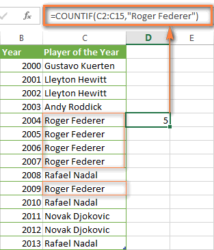
Note. A criterion is case insensitive, meaning that if you type "roger federer" as the criteria in the above formula, this will produce the same result.
Excel COUNTIF function examples
As you have just seen, the syntax of the COUNTIF function is very simple. However, it allows for many possible variations of the criteria, including wildcard characters, the values of other cells, and even other Excel functions. This diversity makes the COUNTIF function really powerful and fit for many tasks, as you will see in the examples that follow.
COUNTIF formula for text and numbers (exact match)
In fact, we discussed the COUNTIF function that counts text values matching a specified criterion exactly a moment ago. Let me remind you that formula for cells containing an exact string of text: =COUNTIF(C2:C15,"Roger Federer"). So, you enter:
- A range as the first parameter;
- A comma as the delimiter;
- A word or several words enclosed in quotes as the criteria.
Instead of typing text, you can use a reference to any cell containing that word or words and get absolutely the same results, e.g. =COUNTIF(C1:C9,C7).
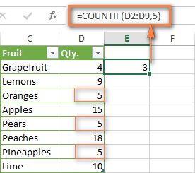
Similarly, COUNTIF formulas work for numbers. As shown in the screenshot below, the below formula perfectly counts cells with quantity 5 in Column D:
=COUNTIF(D2:D9, 5)
In this article, you will find a few more formulas to count cells that contain any text, specific characters or only filtered cells.
COUNTIF formulas with wildcard characters (partial match)
In case your Excel data include several variations of the keyword(s) you want to count, then you can use a wildcard character to count all the cells containing a certain word, phrase or letters as part of the cell's contents.
Suppose, you have a list of tasks assigned to different persons, and you want to know the number of tasks assigned to Danny Brown. Because Danny's name is written in several different ways, we enter "*Brown*" as the search criteria =COUNTIF(D2:D10, "*Brown*").
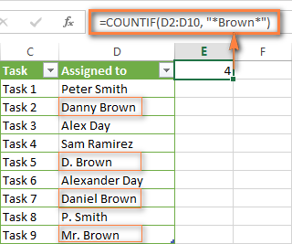
An asterisk (*) is used to find cells with any sequence of leading and trailing characters, as illustrated in the above example. If you need to match any single character, enter a question mark (?) instead, as demonstrated below.
Tip. It is also possible to use wildcards with cell references with the help of the concatenation operator (&). For example, instead of supplying "*Brown*" directly in the formula, you can type it in some cell, say F1, and use the following formula to count cells containing "Brown": =COUNTIF(D2:D10, "*"&F1&"*")
Count cells beginning or ending with certain characters
You can use either wildcard character, asterisk (*) or question mark (?), with the criterion depending on which exactly result you want to achieve.
If you want to know the number of cells that start or end with certain text no matter how many other characters a cell contains, use these formulas:
=COUNTIF(C2:C10,"Mr*") - count cells that begin with "Mr".
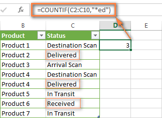
=COUNTIF(C2:C10,"*ed") - count cells that end with the letters "ed".
The image below demonstrates the second formula in action:
If you are looking for a count of cells that start or end with certain letters and contain the exact number of characters, you use the Excel COUNTIF function with the question mark character (?) in the criteria:
=COUNTIF(D2:D9,"??own") - counts the number of cells ending with the letters "own" and having exactly 5 characters in cells D2 through D9, including spaces.
=COUNTIF(D2:D9,"Mr??????") - counts the number of cells starting with the letters "Mr" and having exactly 8 characters in cells D2 through D9, including spaces.
Tip. To find the number of cells containing an actual question mark or asterisk, type a tilde (~) before the ? or * character in the formula. For example, =COUNTIF(D2:D9,"*~?*") will count all cells containing the question mark in the range D2:D9.
Excel COUNTIF for blank and non-blank cells
These formula examples demonstrate how you can use the COUNTIF function in Excel to count the number of empty or non-empty cells in a specified range.
COUNTIF not blank
In some Excel COUNTIF tutorials and other online resources, you may come across formulas for counting non-blank cells in Excel similar to this one:
=COUNTIF(A1:A10,"*")
But the fact is, the above formula counts only cells containing any text values including empty strings, meaning that cells with dates and numbers will be treated as blank cells and not included in the count!
If you need a universal COUNTIF formula for counting all non-blank cells in a specified range, here you go:
Or
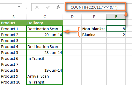
This formula works correctly with all value types - text, dates and numbers - as you can see in the screenshot below.
COUNTIF blank
If you want the opposite, i.e. count blank cells in a certain range, you should adhere to the same approach - use a formula with a wildcard character for text values and with the "" criteria to count all empty cells.
Formula to count cells not containing any text:
Since an asterisk (*) matches any sequence of text characters, the formula counts cells not equal to *, i.e. not containing any text in the specified range.
Universal COUNTIF formula for blanks (all value types):
The above formula correctly handles numbers, dates and text values. For example, here's how you can get the number of empty cells in the range C2:C11:
=COUNTIF(C2:C11,"")
Please be aware that Microsoft Excel has another function for counting blank cells, COUNTBLANK. For instance, the following formulas will produce exactly the same results as the COUNTIF formulas you see in the screenshot above:
Count blanks:
=COUNTBLANK(C2:C11)
Count non-blanks:
=ROWS(C2:C11)*COLUMNS(C2:C11)-COUNTBLANK(C2:C11)
Also, please keep in mind that both COUNTIF and COUNTBLANK count cells with empty strings that only look blank. If you do not want to treat such cells as blanks, use "=" for criteria. For example:
=COUNTIF(C2:C11,"=")
For more information about counting blanks and not blanks in Excel, please see:
COUNTIF greater than, less than or equal to
To count cells with values greater than, less than or equal to the number you specify, you simply add a corresponding operator to the criteria, as shown in the table below.
Please pay attention that in COUNTIF formulas, an operator with a number are always enclosed in quotes.
| Criteria | Formula Example | Description |
|---|---|---|
| Count if greater than | =COUNTIF(A2:A10,">5") | Count cells where value is greater than 5. |
| Count if less than | =COUNTIF(A2:A10,"<5") | Count cells with values less than 5. |
| Count if equal to | =COUNTIF(A2:A10,"=5") | Count cells where value is equal to 5. |
| Count if not equal to | =COUNTIF(A2:A10,"<>5") | Count cells where value is not equal to 5. |
| Count if greater than or equal to | =COUNTIF(C2:C8,">=5") | Count cells where value is greater than or equal to 5. |
| Count if less than or equal to | =COUNTIF(C2:C8,"<=5") | Count cells where value is less than or equal to 5. |
You can also use all of the above formulas to count cells based on another cell value, you will just need to replace the number in the criteria with a cell reference.
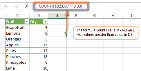
Note. In case of a cell reference, you have to enclose the operator in quotes and add an ampersand (&) before the cell reference. For example, to count cells in the range D2:D9 with values greater than a value in cell D3, you use this formula =COUNTIF(D2:D9,">"&D3):
If you want to count cells that contain an actual operator as part of the cell's contents, i.e. the characters ">", "<" or "=", then use a wildcard character with the operator in the criteria. Such criteria will be treated as a text string rather than a numeric expression. For example, the formula =COUNTIF(D2:D9,"*>5*") will count all cells in the range D2:D9 with contents like this "Delivery >5 days" or ">5 available".
Using Excel COUNTIF function with dates
If you want to count cells with dates that are greater than, less than or equal to the date you specify or date in another cell, you proceed in the already familiar way using formulas similar to the ones we discussed a moment ago. All of the above formulas work for dates as well as for numbers. Let me give you just a few examples:
| Criteria | Formula Example | Description |
|---|---|---|
| Count dates equal to the specified date. | =COUNTIF(B2:B10,"6/1/2014") | Counts the number of cells in the range B2:B10 with the date 1-Jun-2014. |
| Count dates greater than or equal to another date. | =COUNTIF(B2:B10,">=6/1/2014") | Count the number of cells in the range B2:B10 with a date greater than or equal to 6/1/2014. |
| Count dates greater than or equal to a date in another cell, minus x days. | =COUNTIF(B2:B10,">="&B2-"7") | Count the number of cells in the range B2:B10 with a date greater than or equal to the date in B2 minus 7 days. |
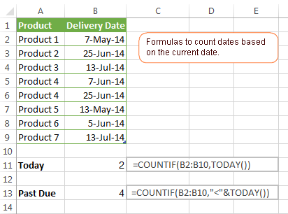
Apart from these common usages, you can utilize the COUNTIF function in conjunction with specific Excel Date and Time functions such as TODAY() to count cells based on the current date.
| Criteria | Formula Example |
|---|---|
| Count dates equal to the current date. | =COUNTIF(A2:A10,TODAY()) |
| Count dates prior to the current date, i.e. less than today. | =COUNTIF(A2:A10,"<"&TODAY()) |
| Count dates after the current date, i.e. greater than today. | =COUNTIF(A2:A10,">"&TODAY()) |
| Count dates that are due in a week. | =COUNTIF(A2:A10,"="&TODAY()+7) |
| Count dates in a specific date range. | =COUNTIF(B2:B10, ">=6/1/2014")-COUNTIF(B2:B10, ">6/7/2014") |
Here is an example of using such formulas on real data (at the moment of writing today was 25-Jun-2014):
Excel COUNTIF with multiple criteria
In fact, Excel COUNTIF function is not exactly designed to count cells with multiple criteria. In most cases, you'd use its plural counterpart, the COUNTIFS function to count cells that match two or more criteria (AND logic). However, some tasks can be solved by combining two or more COUNTIF functions in one formula.
Count values between two numbers
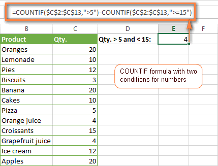
One of the most common applications of Excel COUNTIF function with 2 criteria is counting numbers within a specific range, i.e. less than X but greater than Y. For example, you can use the following formula to count cells in the range B2:B9 where a value is greater than 5 and less than 15.
=COUNTIF(B2:B9,">5")-COUNTIF(B2:B9,">=15")
How this formula works:
Here, we use two separate COUNTIF functions - the first one finds out how many values are greater than 5 and the other one gets a count of values greater than or equal to 15. Then, you subtract the latter from the former and get the desired result.
Count cells with multiple OR criteria
In situations when you want to get several different items in a range, add 2 or more COUNTIF functions together. Supposing, you have a shopping list and you want to find out how many soft drinks are included. To have it done, use a formula similar to this:
=COUNTIF(B2:B13,"Lemonade")+COUNTIF(B2:B13,"*juice")
Please pay attention that we've included the wildcard character (*) in the second criterion, it is used to count all kinds of juice on the list.
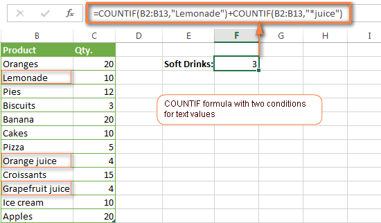
In the same manner, you can write a COUNTIF formula with several conditions. Here is an example of the COUNTIF formula with multiple OR conditions that counts lemonade, juice and ice cream:
=COUNTIF(B2:B13,"Lemonade") + COUNTIF(B2:B13,"*juice") + COUNTIF(B2:B13,"Ice cream")
For other ways to count cells with OR logic, please see this tutorial: Excel COUNTIF and COUNTIFS with OR conditions.
Using COUNTIF function to find duplicates and unique values
Another possible usage of the COUNTIF function in Excel is for finding duplicates in one column, between two columns, or in a row.
Example 1. Find and count duplicates in 1 column
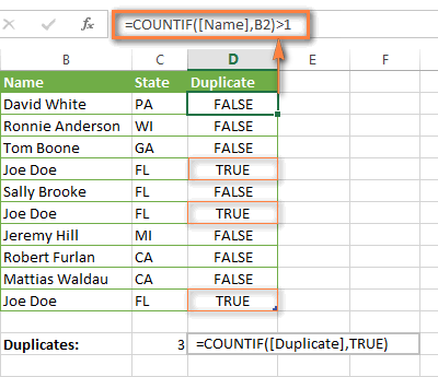
For example, this simple formula =COUNTIF(B2:B10,B2)>1 will spot all duplicate entries in the range B2:B10 while another function =COUNTIF(B2:B10,TRUE) will tell you how many dupes are there:
Example 2. Count duplicates between two columns
If you have two separate lists, say lists of names in columns B and C, and you want to know how many names appear in both columns, you can use Excel COUNTIF in combination with the SUMPRODUCT function to count duplicates:
=SUMPRODUCT((COUNTIF(B2:B1000,C2:C1000)>0)*(C2:C1000<>""))
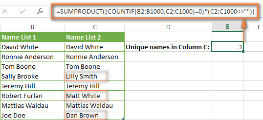
We can even take a step further and count how many unique names there are in Column C, i.e. names that do NOT appear in Column B:
=SUMPRODUCT((COUNTIF(B2:B1000,C2:C1000)=0)*(C2:C1000<>""))
Tip. If you want to highlight duplicate cells or entire rows containing duplicate entries, you can create conditional formatting rules based on the COUNTIF formulas, as demonstrated in this tutorial - Excel conditional formatting formulas to highlight duplicates.
Example 3. Count duplicates and unique values in a row
If you want to count duplicates or unique values in a certain row rather than a column, use one of the below formulas. These formulas might be helpful, say, to analyze the lottery draw history.
Count duplicates in a row:
=SUMPRODUCT((COUNTIF(A2:I2,A2:I2)>1)*(A2:I2<>""))
Count unique values in a row:
=SUMPRODUCT((COUNTIF(A2:I2,A2:I2)=1)*(A2:I2<>""))

Excel COUNTIF - frequently asked questions and issues
I hope these examples have helped you to get a feel for the Excel COUNTIF function. If you've tried any of the above formulas on your data and were not able to get them to work or are having a problem with the formula you created, please look through the following 5 most common issues. There is a good chance that you will find the answer or a helpful tip there.
1. COUNTIF on a non-contiguous range of cells
Question: How can I use COUNTIF in Excel on a non-contiguous range or a selection of cells?
Answer: Excel COUNTIF does not work on non-adjacent ranges, nor does its syntax allow specifying several individual cells as the first parameter. Instead, you can use a combination of several COUNTIF functions:
Wrong: =COUNTIF(A2,B3,C4,">0")
Right: =COUNTIF(A2,">0") + COUNTIF(B3,">0") + COUNTIF(C4,">0")
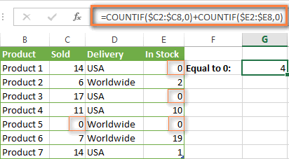
An alternative way is using the INDIRECT function to create an array of ranges. For example, both of the below formulas produce the same result you see in the screenshot:
=SUM(COUNTIF(INDIRECT({"B2:B8","D2:C8"}),"=0"))
=COUNTIF($B2:$B8,0) + COUNTIF($C2:$C8,0)
2. Ampersand and quotes in COUNTIF formulas
Question: When do I need to use an ampersand in a COUNTIF formula?
Answer: It is probably the trickiest part of the COUNTIF function, which I personally find very confusing. Though if you give it some thought, you'll see the reasoning behind it - an ampersand and quotes are needed to construct a text string for the argument. So, you can adhere to these rules:
If you use a number or a cell reference in the exact match criteria, you need neither ampersand nor quotes. For example:
=COUNTIF(A1:A10,10)
or
=COUNTIF(A1:A10,C1)
If your criteria includes text, wildcard character or logical operator with a number, enclose it in quotes. For example:
=COUNTIF(A2:A10,"lemons")
or
=COUNTIF(A2:A10,"*") or =COUNTIF(A2:A10,">5")
In case your criteria is an expression with a cell reference or another Excel function, you have to use the quotes ("") to start a text string and ampersand (&) to concatenate and finish the string off. For example:
=COUNTIF(A2:A10,">"&D2)
or
=COUNTIF(A2:A10,"<="&TODAY())
If you are in doubt whether an ampersand is needed or not, try out both ways. In most cases an ampersand works just fine, e.g. both of the below formulas work equally well.
=COUNTIF(C2:C8,"<=5")
and
=COUNTIF(C2:C8,"<="&5)
3. COUNTIF for formatted (color coded) cells
Question: How do I count cells by fill or font color rather than by values?
Answer: Regrettably, the syntax of the Excel COUNTIF function does not allow using formats as the condition. The only possible way to count or sum cells based on their color is using a macro, or more precisely an Excel User-Defined function. You can find the code working for cells colored manually as well as for conditionally formatted cells in this article - How to count and sum Excel cells by fill and font color.
4. #NAME? error in the COUNTIF formula
Issue: My COUNTIF formula throws a #NAME? error. How can I get it fixed?
Answer: Most likely, you have supplied an incorrect range to the formula. Please check out point 1 above.
5. Excel COUNTIF formula not working
Issue: My COUNTIF formula is not working! What have I done wrong?
Answer: If you have written a formula which is seemingly correct but it does not work or produces a wrong result, start by checking the most obvious things such as a range, conditions, cell references, use of ampersand and quotes.
Be very careful with using spaces in a COUNTIF formula. When creating one of the formulas for this article I was on the verge of pulling my hair out because the correct formula (I knew with certainty it was right!) wouldn't work. As it turned out, the problem was in a measly space somewhere in between, argh... For instance, look at this formula:
=COUNTIF(B2:B13," Lemonade").
At first sight, there is nothing wrong about it, except for an extra space after the opening quotation mark. Microsoft Excel will swallow the formula just fine without an error message, warning or any other indication, assuming you really want to count cells containing the word 'Lemonade' and a leading space.
If you use the COUNTIF function with multiple criteria, split the formula into several pieces and verify each function individually.
And this is all for today. In the next article, we will explore several ways to count cells in Excel with multiple conditions. Hope to see you next week and thanks for reading!
 by
by
1053 comments
Hi!
I need to count the number of countries from a list of employees, excluding those duplicated employees:
For instance, I have three rows with the same employee (190175) from Spain, but I just want it to be counted once based on the empoyee ID.
The formula I have is =COUNTIF($T$2:$T$30,'Spain'), but I dont know how to exclude those duplicated rows with the same ID. Could you help me?
Hello I am trying to write into this equation to IGNORE blanks.
=COUNTIFS(C3:C10000,E3:E10000,D3:D10000,">=5000",A2:A4409,"<=5999")
Any help is appreciated
I want to write the formula for selecting the value of BMI with criteria between 18.5 > 24.9-second criteria for "males". Please guide me.
Hi!
Your problem is not clear to me. Explain in more detail.
Hi Sir, good day.
Can you give me an excel formula on below scenario:
ColumnA-dates
ColumnB-names
I would like to have number of days captured(ColumnA) under specific name(ColumnB).
Thanks!
Hello!
If I got you right, this article will help solve your problem: How to count unique values in Excel with criteria.
If something is still unclear, please feel free to ask.
Vendor - Pay Type
RED - CASH
RED - CASH
BLUE - CHECK
RED - CASH
YELLOW - CASH
BLUE - CHECK
YELLOW - CASH
RED - CASH
I need help figuring out the formula where the end results would be: CASH=2, CHECK=1.
Hello!
Here is the article that may be helpful to you: Count unique values with criteria.
=IFERROR(ROWS(UNIQUE(FILTER(A2:A9,B2:B9="CASH"))), 0)
I just need count one column name and second one is date. name is duplicate in one column but date the increase day by day. I need count between 4 days repeated count.
Name Date
Abc 8/25/2021
BCS 8/25/2021
DEF 8/25/2021
FRG 8/25/2021
ABC 8/22/2021
BCS 8/24/2021
DEF 8/23/2021
FRG 8/21/2021
TYX 8/20/2021
Hi!
Your description is not very clear. What result do you want to get exactly?
Hi!
Im curious about the following scenario:
I have a range of data that will sometimes include blank entries due to an internet intermittent connection. I need to count the number of instances that the data is below a given value, i.e. "<=5". The formula will not count empty cells as being equivalent to zero, and I'm wondering if that has to do with their cell type.
I.e. the cells are currently registered as "General" format, not "Number" format, and I'm wondering if this would change the output of the formula.
I don't want to necessarily change it, but I want to know how I should in case I need to adjust my report.
To reiterate: The formula I am using is registering the cells with values correctly, but the empty cells are acting as a special case, and I want to know how Excel is interpreting their value currently. It is a CountIf formula, not CountA or CountIfs.
Hi!
Excel interprets blank cells as either blank or zero. It depends on the formula. But you did not specify this formula.
Pay attention to the following paragraph of the article above — Count if blank or not blank.
I need to do conditional formatting based upon 2 columns.
I have 4 columns: 'in/out'; 'grade'; 'name'; 'reason'
Basically if someone's name shows up 3 times with each time it shows up with"in" being chosen it needs to be highlighted. if someone's name shows up 3 times with each time it shows up with "in" was only chosenon 1 or two of the times it should not be highlighted
Hi!
Your condition cannot be written using a conditional formatting formula.
Thanks - some great tips.
In a spreadsheet, I want to count if all cells Sheet1!A2:C51514 are blank. When I do this formula =COUNTBLANK(Sheet1!A2:C51514) it seems to add all the blank cells in Sheet1!A2:C51514 together.
BUT I just want to know if ALL three cells in Sheet1!A2:C51514 are blank, not add all the blank cells together.
So when I filter I get 38,538 blanks ie the cells in column A are blank and the cells in column B are blank and the cells in column C are blank. This is the right number because it is not adding the blank cells together.
=COUNTBLANK(Sheet1!A2:C51514) gives me 141,116.
Do you know a formula to count if all the cells (A2:C51514) are blank?
Should I use =SUMPRODUCT((COUNTIF(Sheet1!(A2:A51514)=” “)+(COUNTIF(Sheet1!(A2:A51514)=” “) ?
Hello!
If I got you right, the formula below will help you with your task:
=COUNTIFS(A1:A10,"",B1:B10,"",C1:C10,"")
Read the article - How to use Excel COUNTIFS and COUNTIF with multiple criteria
i want to count the words like {"PL","HOL","CFL"} as 1 and {"HD","CFL-HD" } as .5 appearing in a row if the date on the other row is greater than today()
also if the date is less than today()
=SUM(COUNTIFS($C$1:$AG$1,"="&TODAY(),$C$2:$AG$2,{"PL","HOL","CFL"}))
Hello!
If I understand your task correctly, the following formula should work for you:
=SUM(COUNTIFS($C$1:$AG$1,">"&TODAY(),$C$2:$AG$2,{"PL","HOL","CFL"}))+SUM(COUNTIFS($C$1:$AG$1,">"&TODAY(),$C$2:$AG$2,{"HD","CFL-HD"}))*0.5
I hope this will help.
Good day
Please please assist
I am trying to sum up the hours lost due breakdown or other reason in that particular reasons column.
Column B: shifts, either morning, afternoon or night shift
Column k: time they actually started work
Column L: reason of starting late like breakdown
Morning shift suppose to start work at 08:30, and afternoon shift 14:30 and night shift 21:30
I'm trying to get hours lost per particular reason.
Hello!
Please have a look at this article — Calculate time in Excel, time difference
For example,
=SUM(K2:K100-TIME(8,30,0))
or
=SUMPRODUCT((K2:K100-TIME(8,30,0)),--(L2:L100="reason 1"))
I hope my advice will help you solve your task.
Hi Alex
Is basically counting the "blanks" at "L" if the the time at "k" more than required(08:30, 14:30 and 20:30)
kind regards
Thank Alex
Please assist I am trying to identify reason for late start, and where there is late start but no reason booked, hence I want to count the blanks if the start up was greater than require of 08:30, 14:30 and 20:30 in different shifts.
Time should be greater than 08:30 and less than 13:00, and greater than 14:30 and less than 18:00 and also greater than 20:30 and less than 23:00
Column B
shift
Morning/Afternoon/Night
Column k
Time
Column L
reasons for late start and Blanks that I want to count
Hi!
Add another condition to the COUNTIFS formula.
=COUNTIFS(B2:B5,">"&TIME(8,30,0),B2:B5,"<"&TIME(13,0,0),C2:C5,"")
May you please assist me.
I have blank rows with data and without data, which were suppose to be having data.
I want to count the blank rows if the time is greater than e.g 08:30
* e.g: countblank C5, if B5 Is greater than 08:30
Hello!
I recommend reading this guide: Excel COUNTIFS and COUNTIF with multiple AND / OR criteria.
Please try the following formula:
=COUNTIFS(B2:B5,">"&TIME(8,30,0),C2:C5,"")
or
=SUMPRODUCT(--(B2:B5>TIME(8,30,0)),--(C2:C5=""))
Hello,
I encountered this problem with countif function: if in one cell I have the value "5" and in another one "05" it sees them as duplicates. Is there any way to write the function so it doesn't see them as duplicates?
Thank you
Hello!
You have not written what condition you use in the COUNTIF function. Therefore, I cannot give you an exact answer.
I would advise you to check that 5 and 05 are written as text. I assume that 5 is written as a number.
Describe in detail what problem you have, and I will try to help you.
i want to count only in my data if country =" USA" in one column and state = " Califrornia" in other column.
Hello!
Here is the article that may be helpful to you: How to use Excel COUNTIFS and COUNTIF with multiple criteria
I am trying to use countif based on certain criteria.
I have 20 provider names. Each name may be assigned 100 patients. I need to count how many orders that physician entered per patient. Sometimes there are no orders at all. The orders are time stamped by date and time. I need to count the date/time for each specific provider. The date range anywhere between 1/1/2021 00:01 to 3/31/2021 23:59. I tried to just use count A but I wasn't sure how to to use that with Countif
I am thinking
=countif(range=name, range,_____)
I not sure what to specify for my 2nd range.
Thanks!
Hello!
Please check out the following article on our blog, it’ll be sure to help you with your task: Excel COUNTIFS with multiple AND / OR criteria.
I hope I answered your question. If something is still unclear, please feel free to ask.
Hello,
I want to use a formula in excel to return the number of "Yes" results in a range, with the result of each inquiry returning either zero (there are zero yes results), or 1 if there is 1 or more of entries of "Yes" in the range.
Is that possible? I assume use Countif with some additional formula?
Hi,
If I understand your task correctly, the following formula should work for you:
=COUNTIF(A1:D50,"Yes")
If this is not what you wanted, please describe the problem in more detail.
Hi,
How to COUNTIF specific model (eg. CHEVY) which had expired last 2 weeks (let's say the date today is 01-Mar-21). Moreover, the result will be on another sheet. tnx.
MODEL Registration# Reg. Date Expiry Date
CHEVY 313001 03-Jan-20 03-Feb-21
TAHOE 314001 10-Jan-20 10-Jan-22
CAMRY 315001 17-Jan-20 17-Jan-22
CHEVY 313002
LIBERTY 316001 01-Feb-20 01-Feb-21
TAHOE 314002 08-Feb-20 08-Feb-21
CHEVY 313004 29-Feb-20 29-Feb-21
TAHOE 314003 15-Feb-20 15-Feb-21
CHEVY 313003
CHEVY 313005 29-Feb-20 28-Feb-21
TAHOE 314004 15-Feb-20 15-Feb-21
CHEVY 313006 29-Feb-20 25-Feb-21
Hi,
The formula below will do the trick for you:
=COUNTIFS(A1:A12,"CHEVY",D1:D12,">"&TODAY()-14,D1:D12,"<"&TODAY())
You can learn more about COUNTIFS in Excel in this article on our blog.
I want to count number of cells in Google Sheet only when another cell contains some text.
Customer Name
Total Time
Work Start Work End 00:00
Team Used
Van 1 Van 2 Team Size
Sr. No. Name Site Name Name 7
1 Rahul Patil Weekly Off Vikas Wakude
2 Pradip Vetal Weekly Off Harish Wakude Van1 4
3 Vijay Patil Weekly Off Suresh Salunkhe Van2 1
4 Vikas Wakude Weekly Off
For e.g. I want to count " Name " only when " Customer Name " contains some text.
Please help.
Thanks.
Hi There
I have a column containing over 1,000 entries of about 200 company names. I want to count the number of times each company name occurs. How do I do this?
I'd like to save the result in a new sheet.
Any idea? Thanks for your help.
Anna O.
Hello!
You can get a list of unique values using the UNIQUE function. You can count how many times each name occurs using the COUNTIF function.
I hope I answered your question. If something is still unclear, please feel free to ask.
How to packets counts row numbers multiple other row formula
Hi!
What do you want to calculate exactly? Your question is not entirely clear, please specify.
Can Countif be used with a function in the criteria? My column O has dates. I want to count how many dates are in 2020. I tried something like =COUNTIF(YEAR(O8:O609),"=2020") and =COUNTIF(O8:O609,"YEAR()=2020")
Hello!
Please try the following formula:
=SUM(--(YEAR(O8:O609)=2020))
COUNTIF does not work with arrays, so cannot be used YEAR(O8:O609)
I hope I answered your question. If something is still unclear, please feel free to ask.
I have built a complicated spreadsheet in Google Sheets containing several SUMIF uses. Is there an easy way to add column next to the resulting column giving the number of cells counted in each resulting cell in this resulting column? Here is an example of a cell which is a part of a column of formuli. I want to place another column the the right of this column showing the number of cells which were counted to make the results in the cell to its left.
=SUMIF(D$10:D$110, AA23, C$10:C$110)
Thank you for your help.
Hello!
If I understand you correctly, you can use the COUNTIF function with the same arguments as in SUMIF.
=COUNTIF(D$10:D$110, AA23, C$10:C$110)
I hope my advice will help you solve your task.
Hi There,
I have a column say "A" filled with data. I need a combination of formulas (IF & COUNTIF) on column B to validate firstly that if the cell A is blank, the result is blank. Else, if there is a value, it validates all of column A for duplicates and highlights for "Duplicates", else the result is "Unique". Can you please help?
Hello!
Please use the following formula/the formula below to solve your task:
=IF(A2="","",IF(COUNTIF($A$2:$A$10,B2)>1,"Duplicate","Unique"))
I hope this will help
Below formula is working for I,J,K and L. Except if i put range then the formula breaks.
Working:
=SUM((TRIM(I153)"")*(TRIM(K153)"")*(TRIM(L153)"")*(TRIM(J153)""))
Not Working:
=SUM((TRIM(I2:I153)"")*(TRIM(K2:K153)"")*(TRIM(L2:L153)"")*(TRIM(J2:J153)""))
Hi,
I gave you another formula. These formulas cannot work.
I have a formula which seems to be working ok. My formula is to check the columns I,J,K,L cannot be a blank. I am using below. I column is text, K column is text, L column is text and J column is a list.
=COUNTIFS(I2:I153,"",K2:K153,"",L2:L153,"")+COUNTIF(J2:J153,"0,1,N/A")
if the criteria is matched then it is counted as a verified row.
Users are giving a space I OR K OR L which seems to be counting as non-blank and making it as a verified row with no data that makes sense.
Is there a way to not to count a space as valid entry or just no count if only space is provided in the column.
Many thanks in advance
actually the formula is this. above question have incorrect formula.
=COUNTIFS(I2:I153,"",K2:K153,"",L2:L153,"")+COUNTIF(J2:J153,"0,1,N/A")
Hello!
If I understand your task correctly, the following formula should work for you:
=SUM((TRIM(I2:I153)="")*(TRIM(K2:K153)="")*(TRIM(L2:L153)=""))+COUNTIF(J2:J153,"0,1,N/A")
I'm not sure if COUNTIF(J2:J153,"0,1,N/A") is written correctly. But I do not have your data and I cannot check the condition "0,1,N/A". I think it should be 3 conditions.
I hope this will help, otherwise please do not hesitate to contact me anytime.
Thank you Alexander for your reply.
I need more help. You may have understood other way around. Sorry about not to be so clear.
For example there columns I,J,K,L
Criteria 1 is: I, J, K and L cannot be empty. Must have at least one character, not just spaces allowed.
Your formula worked for 3 columns if i made a change like below.
=SUM((TRIM(I153)"")*(TRIM(K153)"")*(TRIM(L153)""))
However range is not working. Getting #value error.
The j column must have a value 0 or 1 or N/A. User will be provided an excel sheet with to select from a list 0,1,N/A.
Formula in text:
Columns I2 to I153 must have at least one character (no space) and K2 to K153 (event better if it is a date) must have at least one character and L2 to L153 (no space) must have at least one character and J2 to J153 must select a value 0,1,N/A.
Hope I am clear on my question.
Thank you again for your time helping me in this.
Hi,
The formula I sent to you was created based on the description you provided in your first request. However, as far as I can see from your second comment, your task is now different from the original one.
If data in column J is selected from a list and cannot be entered manually, then only non-blank cells can be counted.
The formula counts the number of rows that have at least one blank cell.
=SUM(--(((TRIM(I2:I153)="")+(TRIM(K2:K153)="")+(TRIM(L2:L153)="")+(TRIM(J2:J153)=""))>0))
I hope it’ll be helpful.
I have COUNTIFS(H34:AI34,"OFF" in attendance schedule so with the same range i dont want to count "AL" please give me formula where i can put multiple condition.
For Example
Range is H34:AI34
Criteria is OFF and AL which mean i dont want to count OFF and AL
Hello!
The COUNTIFS function uses several conditions. Please check out the following article on our blog, it’ll be sure to help you with your task: Excel COUNTIFS and COUNTIF with multiple AND / OR criteria
I hope this will help.
Hi
I have a list where I need to count the number of records which meet a 2 criteria.
Application name and Critical or Non Critical
The application name is contained in a string of text the Critical/Non Critical is in a separate cell.
Column A, the status Critical or Non Critical is in Column B
Column A contains one of the following
Security Global
Security Global AS400
Security Global Link
Security Global Unix / Linux
Security Global Windows
Security Global z/OS
Column B is either
Critical
Non Critical
I have a formula to count the entries for "AS400", "Link", "Windows" etc
=COUNTIFS($A$2:$A$14,"*AS400*",$B$2:$B$14,"Critical")
but if I search for Global it brings back everything.
=COUNTIFS($A$2:$A$14,"*Global*",$B$2:$B$14,"Non Critical")
Is there an easy way to get it to count the cells which contain just "Global" and not include the "Global Windows" etc
Many thanks in advance
Hello!
If I understand your task correctly, the following formula should work for you:
=COUNTIFS($A$2:$A$14,"*Global*",$B$2:$B$14,"Non Critical",$A$2:$A$14,"<>"&"*Global Windows*")
Hope this is what you need.
Hello,
I have a report that I am trying to figure out a formula for. I am using a countifs formula that has several ranges and criteria. The report has a 1 in every cell of column A, employee name in column B, date of first day in quarantine in column C, date of last day in quarantine in column D, either a 0 or 1 in column E (0=quarantine and 1=positive test and quarantine) and the final few columns are irrelevant to the formula. The information I am looking for is: 1) total positive test/quarantines, 2) total overall quarantine, 3) total 14 day quarantine based on dates in column C and D, 4) total 10 day quarantine based on dates in column C and D. The formula I am using for the each is as follows:
1) =countif(E2:E800, "1") - correct total
2) =countifs(A2:A800, "1", C2:C800, ">="&TODAY()-"14", D2:D800, "="&TODAY()-"14", D2:D800, "="&TODAY()-"10", D2:D800, "<="&TODAY()+"10")
The current total number of employees in quarantine is 7, but the formula is giving 14 which is the total number of employees that are in quarantine based on the date in column C only rather than counting if the dates meet the criteria for both columns C and D. How do I get the formula to consider the second range and criteria when counting? I thought countif functions recognized "and" rather than "or" in the format I am using.
Hello!
I cannot validate the formula without your data, but I recommend trying the formula
=countifs(A2:A800, 1, C2:C800, ">="&(TODAY()-14), D2:D800, “=”&(TODAY()-14), D2:D800, “=”&(TODAY()-10), D2:D800, “<="&(TODAY()+10))
I hope I answered your question. If something is still unclear, please feel free to ask.
Dear All,
I want to calculate no. years month and days to calculate experience tenure and then calculate that experience with 4:1 ratio please suggest formula anyone.
Hello!
To calculate the number of months and years, I recommend using this guide: DATEDIF - calculating date difference in days, weeks, months.
I hope this will help.
Hi,
I have a problem for the last criteria. the criteria should be the value of AO is less than AJ. below is my code.
Sheets("Visual Data (materials)").Cells(33, i) = Application.WorksheetFunction.SumIfs(Sheets("Raw Data (Materials)").Range("AS:AS"), Sheets("Raw Data (Materials)").Range("C:C"), "GEN", Sheets("Raw Data (Materials)").Range("AK:AK"), ">=1/1/" & Sheets("Visual Data (materials)").Cells(32, i), Sheets("Raw Data (Materials)").Range("AK:AK"), "<=12/31/" & Sheets("Visual Data (materials)").Cells(32, i), Sheets("Raw Data (Materials)").Range("AO:AO"), Sheets("Raw Data (Materials)").Range("AO:AO") & "<" & Sheets("Raw Data (Materials)").Range("AJ:AJ"))
Hello!
It is very difficult to understand a formula that contains unique references to your workbook worksheets. Hence, I cannot check its work, sorry.
my question is actually, how can I include a criteria for countifs where values in range A:A is less than range B:B
Hi,
The formula will work. If these are ranges for criteria, then only data for which the conditions are met in two ranges at the same time will be counted.
My question is simple but I don't know what formula to use to make it happen. I'm a quilter. There are a number of squares I get in a package of fabric squares to sew together to make a quilt. I would like a formula that I can put in the number of squares I have in a certain design and have it tell me how many different combinations of rows and columns I could have. Then show me in a diagram.
This kind of formula is beyond my skill level. So if anyone would like to figure this out for me, I would definitely appreciate it!! Thanks!!
Hi!
How do I calculate a count of cells, omitting only the duplicates. that is, if there are 10 entries, and 2 of them appear twice, it should return an answer of 8 (not 6 or 4)?
thank you!
Hello!
You can learn more about counting unique values in Excel in this article on our blog.
I hope I answered your question. If something is still unclear, please feel free to ask.
How do I insert a VLOOKUP as the criteria
I tried but it keeps failing
For example :-
=COUNTIF($G5:DR5,"<VLOOKUP(A5,Codes!$A:$E,4,0)")
Hello!
It is not possible to insert VLOOKUP as a less than criterion in the COUNTIFS function.
I recommend using something like this formula
=SUM(--($G5:$DR5<VLOOKUP($A$5,Codes!$A:$E,4,FALSE)))
I hope it’ll be helpful.
Thank you :)
But i did figure out to insert a VLOOKUP as a criteria and it worked
=COUNTIF($G5:DR5,"<"&VLOOKUP(A5,Codes!$A:$E,4,0))
The formula that I'm using is =COUNT(E143:E419)+COUNT(G143:G419) for the entry's and the =COUNTIFS(F143:F419;">=8:00")+COUNT(H143:H419) and in the result cell is =MAX(0;N1-O1) but it limits the leaving to 8:00 am, do you have a solution for this? Sorry for the bad english
Hello!
It is difficult to give advice without seeing your data. But perhaps the instruction will be useful to you - COUNTIF formulas for dates.
Also, I do not know in what format your time is written. But you need to use the TIME function. Instead of ”>=8:00″, use >TIME(8,0,0). I suggest you read this article.
Thank you, I will take a look
Hi
I need to count the number is cars that are present inside a parking lot. The trick is that sometimes some cars enter the day before and the record is for a single day. I need to count only the entry's but not when it leaves, but I still need to register the hour he leaves. So one camp as the license plate and then the entry hour and the leaving hour, I need to count the leaving hour but only if he has a entry ou else ignore or return a 0 but still count all the others cars inside!
How can one count the number of cells in column A in which the values are greater than the corresponding values in column B? What Excel command should I use? I tried sumproduct but it isn't applicable as it adds up the actual values whereas I only want to know how many cells in A have values greater than B. Thanks.
Hello!
If I understand your task correctly, the following formula should work for you:
=SUM(--(A1:A20>B1:B20))
Hope this is what you need.
hi , I really need help , is there a way that I can count text that is in a range but not part of my "List" for example i had people fill a survey one of the qeustions had multiple checkboxes , the one checkbox was open awnser so i want to count the awnsers that are not in the pre specified checkboxes the [] other:_____ text I hope that this makes some sense to someone
Hello!
Without seeing your data, I cannot write a formula for you. But please reread the article above, it covers your case completely.
I am doing a COUNTIF formula =COUNTIF($C$5:$C$19,"ben*"), but I need to copy the formula to three other cells. When I copy them, the exact same formula comes up for each line, but I need the "ben*" to change each time to a different name (cap, cat, hun). How do I get my formula to recognize that it needs to change without doing it manually?
Hello!
Instead of “ben *”, write a reference to the cell with this value in the formula. Like this:
=COUNTIF($C$5:$C$19,D1)
When you copy a formula, the link will change to a different cell.
How do I count those records where Column X is not blank AND Column Y is blank? For example, Column X is "Drafts Uploaded" and Column Y is "Shipped." I need to count those record for which drafts were uploaded (Column X is not blank) but have NOT been shipped (Column Y is blank).
Hello!
You have 2 conditions. Read in this article how to count cells with multiple criteria.
what a formula be to count a range of blank cells if filtered.
Ex. have a list, only want to count blank cells. If i only want the blank cells when i filter NY, how can i get it to only count the blank cells when i filter
Hello!
In the instructions above, read the "COUNTIF blank" section.
I have a lengthy list of names with dollars tied to purchases to each of those names. I am attempting to add up the totals for each of the individuals. Some have 3 lines, some have 1 and others have 5. How would I go about getting this to work?
Hello!
Unfortunately, without seeing your data it hard to give you advice. For me to be able to help you better, please describe your task in more detail. Please specify what you were trying to find, what formula you used and what problem or error occurred. Give an example of the source data and the expected result.
It’ll help me understand it better and find a solution for you.
How do you use countif when the cells you want to count have a return value in the Dated format example below.
4 Yrs, 11 Mths & 8 Days
The above shows length of service the formula used is:
=IFERROR(IF(E6="","",DATEDIF(E6,$C$2,"y") & " Yrs, " & DATEDIF(E6,$C$2,"ym") & " Mths & " & DATEDIF(E6,$C$2,"md") & " Days "),"")
Now I want to count how many colleagues have a length of service of more that 3 yrs. Is that possible?
Thanks
Phil
Hello!
You can count the number of dates for which the difference is more than 36 months:
=SUM(--(DATEDIF($E$1:$E$10,$C$2,"m")>36))
I hope this will help, otherwise please do not hesitate to contact me anytime.
I want to count alternate column value. for example i have column A-B-C-D but i need only to count column A & C Value.Please help me to know how i can do by formula.
Hello!
You did not say by what criteria you will count. Therefore, I cannot give an exact recommendation. However, you can add the two COUNTIF functions. In the first you count by column A, in the second you count by column C. Or you can use the COUNTIFS function. Read more here.
Help me, how to calculate duplicate value for below range? i notice when i use this coding, repeated values such as 93 twice, not counted.
=COUNTIFS(Z5:Z14,">=90",Z5:Z14,"<=94")
Thanks in advance
I want to count the no of cell with a particular value in continuation and break the counting is that value changes in a cell. which formula I have to use ?
SEGMENT NAME 20Jul 21Jul 22Jul 23Jul 24Jul 25Jul 26Jul 27Jul 28Jul 29Jul Desired count reslut (Count <1)
GOMADBAMANN3 100.00 96.61 76.37 19.06 9.25 0.00 90.24 0.00 0.72 0.00 2
GOMADBAMANN1 100.00 96.07 76.37 20.99 39.14 86.97 99.94 0.00 76.60 0.00 1
GOMADBAMANN2 100.00 96.76 76.37 15.67 0.04 52.55 0.00 82.61 78.17 0.00 1
GOKILKILLIS3 100.00 99.97 100.00 100.00 100.00 97.25 0.00 73.75 33.04 0.00 1
GOKILKILLIS4 100.00 99.97 100.00 100.00 100.00 97.22 0.00 75.06 33.03 0.00 1
GOPARMADHAI1 0.00 36.65 19.06 0.00 0.00 0.00 0.00 0.00 0.00 0.00 7
GOPARMADHAI2 0.00 36.65 19.06 0.00 0.00 0.00 0.00 0.00 0.00 0.00 7
GOPARMADHAI3 0.00 36.65 19.06 0.00 0.00 0.00 0.00 0.00 0.00 0.00 7
GOAMRAMRMAS3 100.00 100.00 100.00 100.00 100.00 0.00 0.00 100.00 34.87 0.00 1
GOJADJADAUD1 0.00 0.00 0.00 0.00 0.00 0.00 0.00 0.00 0.00 0.00 10
GOJADJADAUD2 0.00 0.00 0.00 0.00 0.00 0.00 0.00 0.00 0.00 0.00 10
GOJADJADAUD3 0.00 0.00 0.00 0.00 0.00 0.00 0.00 0.00 0.00 0.00 10
GOHINHINDXX2 99.65 99.24 99.18 99.53 5.48 56.80 99.02 98.91 41.28 0.00 1
GOBELBELA1X1 0.31 0.00 0.00 0.91 0.58 0.11 0.80 2.67 0.00 0.00 2
GOFIRSADABA1 99.74 99.66 99.58 99.85 99.74 0.00 0.00 100.00 100.00 0.00 1
GOFIRSADABA2 99.74 99.65 99.58 99.92 99.74 0.00 0.00 100.00 100.00 0.00 1
0100000037 288.00 288.00 PCS TRUE
0100000037 234.00 234.00 PCS TRUE
0100000037 384.00 384.00 PCS TRUE
0100000038 36.00 36.00 PCS TRUE
0100000038 24.00 24.00 PCS TRUE
0100000041 120.00 120.00 PCS TRUE
0100000041 120.00 120.00 PCS TRUE
0100000044 168.00 168.00 PCS TRUE
0100000044 108.00 108.00 PCS TRUE
0100000045 144.00 144.00 PCS TRUE
0100000047 240.00 240.00 PCS TRUE
What formula should i use to count every cell ?
for example 0100000037 this Code is showing in 3 cells so what i ll do to calculate in cell a1=1 a2=2 a3=3 and so and so ?
The "COUNTIF - COUNTIF to count numbers within a range" section is clearly wrong. If you just manually count the matches on the list, there are a total of 5.
Not sure if your understanding of the function is wrong or just your visual aid, but since I can't get this to work based on your instruction I suspect it is the former.
Hello Charles!
You're right - the formula does not take into account the number 15. Thank you for your attention. I fixed everything
Count in a single formula total A or B Or C
where =COUNTIF(C1,"A") it can count only A