This tutorial explains the difference between the SUMIF and SUMIFS functions in terms of their syntax and usage, and provides a number of formula examples to sum values with multiple AND / OR criteria in Excel 365, 2021, 2019, 2016, 2013, 2010, and lower.
As everyone knows, Microsoft Excel provides an array of functions to perform various calculations with data. A few articles ago, we explored COUNTIF and COUNTIFS, which are designed for counting cells based on a single condition and several conditions, respectively. Last week we covered Excel SUMIF that adds values meeting the specified criteria. Now it's time to go over the plural version of SUMIF - Excel SUMIFS that allows summing values by multiple criteria.
Those who are familiar with the SUMIF function might think that converting it to SUMIFS takes just an extra "S" and a few additional criteria. This would seem quite logical… but "logical" it's not always the case when dealing with Microsoft : )
Excel SUMIF function - syntax & usage
The SUMIF function is used to conditionally sum values based on a single criteria. We discussed the SUMIF syntax in detail in the previous article, and here's just a quick refresher.
- range - the range of cells to be evaluated by your criteria, required.
- criteria - the condition that must be met, required.
- sum_range - the cells to sum if the condition is met, optional.
As you see, the syntax of the Excel SUMIF function allows for one condition only. And still, we say that Excel SUMIF can be used to sum values with multiple criteria. How can that be? By adding the results of several SUMIF functions and by using SUMIF formulas with array criteria, as demonstrated in the examples that follow.
Excel SUMIFS function - syntax & usage
You use SUMIFS in Excel to find a conditional sum of values based on multiple criteria. The SUMIFS function was introduced in Excel 2007 and is available in all subsequent versions of Excel 2010, 2013, 2016, 2019, 2021, and Excel 365.
Compared to SUMIF, the SUMIFS syntax is a little bit more complex:
The first 3 arguments are mandatory, additional ranges and their associated criteria are optional.
sum_range- one or more cells to sum, required. This can be a single cell, a range of cells or a named range. Only cells with numbers are summed; blank and text values are ignored.criteria_range1- the first range to be evaluated by the associated criteria, required.criteria1- the first condition that must be met, required. You can supply the criteria in the form of a number, logical expression, cell reference, text or another Excel function. For example you can use criteria such as 10, ">=10", A1, "cherries" or TODAY().criteria_range2, criteria2, …- these are additional ranges and criteria associated with them, optional. You can use up to 127 range/criteria pairs in SUMIFS formulas.
Notes:
- For a SUMIFS formula to work correctly, all the criteria_range arguments must have the same dimension as sum_range, i.e. the same number of rows and columns.
- The SUMIFS function works with AND logic, meaning that a cell in the sum range is summed only if it meets all of the specified criteria, i.e. all the criteria are true for that cell.
Basic SUMIFS formula
And now, let's have a look at the Excel SUMIFS formula with two conditions. Suppose, you have a table listing the consignments of fruit from different suppliers. You have the fruit names in column A, suppliers' names in column B, and quantity in column C. What you want is to find out a sum of amounts relating to a given fruit and supplier, e.g. all apples supplied by Pete.
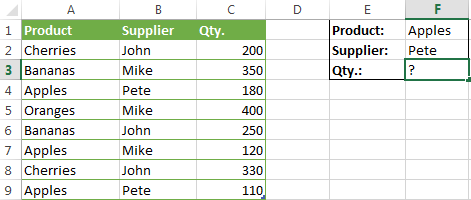
When you're learning something new, it's always a good idea to start with simple things. So, to begin with, let's define all the arguments for our SUMIFS formula:
- sum_range - C2:C9
- criteria_range1 - A2:A9
- criteria1 - "apples"
- criteria_range2 - B2:B9
- criteria2 - "Pete"
Now assemble the above parameters, and you will get the following SUMIFS formula:
=SUMIFS(C2:C9, A2:A9, "apples", B2:B9, "Pete")
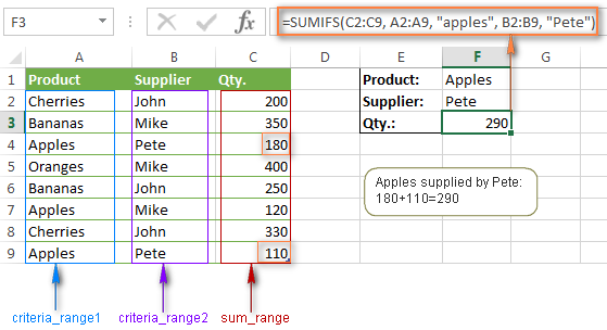
To refine the formula further, you can replace the text criteria "apples" and "Pete" with cell references. In this case, you won't have to change the formula to calculate the quantity of other fruit from a different supplier:
=SUMIFS(C2:C9, A2:A9, F1, B2:B9, F2)
Note. Both the SUMIF and SUMIFS functions are case-insensitive by nature. To get them to recognize the text case, please see Case-sensitive SUMIF and SUMIFS formula in Excel.
SUMIF vs. SUMIFS in Excel
Since the aim of this tutorial is to cover all possible ways to sum values by several conditions, we will discuss formula examples with both functions - Excel SUMIFS and SUMIF with multiple criteria. To use them correctly, you need to clearly understand what these two functions have in common and in what way they are different.
While the common part is clear (similar purpose and parameters), the differences are not so obvious, though very essential.
There are 4 major differences between SUMIF and SUMIFS:
- Number of conditions. SUMIF can evaluate just one condition at a time while SUMIFS can check for multiple criteria.
- Syntax. With SUMIF, the sum_range is the last and optional argument - if not defined, the values in the range argument are summed. With SUMIFS, sum_range is the first and required argument.
- Size of ranges. In SUMIF formulas, sum_range does not necessarily have to be of the same size and shape as range, as long as you have the top left cell right. In Excel SUMIFS, each criteria_range must contain the same number of rows and columns as the sum_range argument.
For example, SUMIF(A2:A9,F1,C2:C18) will return the correct result because the leftmost cell in the sum_range argument (C2) is right. So, Excel will make the correction automatically and include as many columns and rows in sum_range as there are in range.
A SUMIFS formula with unequally sized ranges will return a #VALUE! error.
- Availability. SUMIF is available in all Excel versions, from 365 through 2000. SUMIFS is available in Excel 2007 and higher.
Alright, enough strategy (i.e. theory), let's get into the tactics (i.e. formula examples : )
How to use SUMIFS in Excel - formula examples
A moment ago, we discussed a simple SUMIFS formula with two text criteria. In the same manner, you can use Excel SUMIFS with multiple criteria expressed by numbers, dates, logical expressions, and other Excel functions.
Example 1. Excel SUMIFS with comparison operators
In our fruit suppliers table, suppose, you want to sum all deliveries by Mike with Qty. 200 or more. To do this, you use the comparison operator "greater than or equal to" (>=) in criteria2 and get the following SUMIFS formula:
=SUMIFS(C2:C9,B2:B9,"Mike",C2:C9,">=200")
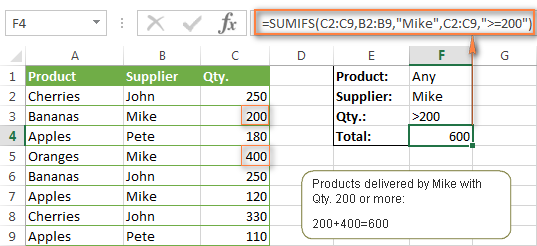
Note. Please pay attention that in Excel SUMIFS formulas, logical expressions with comparison operators should always be enclosed in double quotes ("").
We covered all possible comparison operators in detail when discussing Excel SUMIF function, the same operators can be used in SUMIFS criteria. For example, the following formula with return the sum of all values in cells C2:C9 that are greater than or equal to 200 and less than or equal to 300.
=SUMIFS(C2:C9, C2:C9,">=200", C2:C9,"<=300")
Example 2. Using Excel SUMIFS with dates
In case you want to sum values with multiple criteria based on the current date, use the TODAY() function in your SUMIFS criteria, as demonstrated below. The following formula sums values in column D if a corresponding date in column C falls within the last 7 days, including today:
=SUMIFS(D2:D10, C2:C10,">="&TODAY()-7, C2:C10,"<="&TODAY())
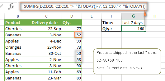
Note. When you use another Excel function together with a logical operator in the criteria, you have to use the ampersand (&) to concatenate a string, for example "<="&TODAY().
In a similar fashion, you can use the Excel SUMIF function to sum values in a given date range. For example, the following SUMIFS formula adds the values in cells C2:C9 if a date in column B falls between 1-Oct-2014 and 31-Oct-2014, inclusive.
=SUMIFS(C2:C9, B2:B9, ">=10/1/2014", B2:B9, "<=10/31/2014")
The same result can be achieved by calculating the difference of two SUMIF functions, as demonstrated in this example - How to use SUMIF to sum values in a given date range. However, Excel SUMIFS is much easier and more understandable, isn't it?
Example 3. Excel SUMIFS with blank and non-blank cells
When analyzing reports and other data, you may often need to sum values corresponding either to empty or non-empty cells.
| Criteria | Description | Formula Example | |
|---|---|---|---|
| Blank cells | "=" | Sum values corresponding to blank cells that contain absolutely nothing - no formula, no zero length string. | =SUMIFS(C2:C10, A2:A10, "=", B2:B10, "=")
Sum values in cells C2:C10 if the corresponding cells in columns A and B are absolutely empty. |
| "" | Sum values corresponding to "visually" blank cells including those that contain empty strings returned by some other Excel function (for example, cells with a formula like =""). | =SUMIFS(C2:C10, A2:A10, "", B2:B10, "")
Sum values in cells C2:C10 with the same conditions as the above formula, but includes empty strings. |
|
| Non-blank cells | "<>" | Sum values corresponding to non-empty cells, including zero length strings. | =SUMIFS(C2:C10, A2:A10, "<>", B2:B10, "<>")
Sum values in cells C2:C10 if the corresponding cells in columns A and B are not empty, including cells with empty strings. |
| SUM-SUMIF or SUM / LEN |
Sum values corresponding to non-empty cells, not including zero length strings. | =SUM(C2:C10) - SUMIFS(C2:C10, A2:A10, "", B2:B10, "")
=SUM((C2:C10) * (LEN(A2:A10)>0)*(LEN(B2:B10)>0)) Sum values in cells C2:C10 if the corresponding cells in columns A and B are not empty, cells with zero length strings are not included. |
And now, let's see how you can use a SUMIFS formula with "blank" and "non-blank" criteria on real data.
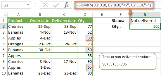
Suppose, you have an order date in column B, delivery date in column C and Qty. in column D. How do you find the total of products that have not been delivered yet? That is, you want to know the sum of values corresponding to non-empty cells in column B and empty cells in column C.
The solution is to use the SUMIFS formula with 2 criteria:
=SUMIFS(D2:D10, B2:B10,"<>", C2:C10,"=")
Using Excel SUMIF with multiple OR criteria
As noted in the beginning of this tutorial, the SUMIFS function is designed with AND logic. But what if you need to sum values with multiple OR criteria, i.e. when at least one of the conditions is met?
Example 1. SUMIF + SUMIF
The simplest solution is to sum the results returned by several SUMIF functions. For example, the following formula demonstrates how to find the total of products delivered by Mike and John:
=SUMIF(C2:C9,"Mike",D2:D9) + SUMIF(C2:C9,"John",D2:D9)
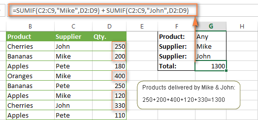
As you see, the first SUMIF function adds the quantities corresponding to "Mike", the other SUMIF function returns the amounts relating to "John" and then you add these 2 numbers.
Example 2. SUM & SUMIF with an array argument
The above solution is very simple and may get the job done quickly when there are only a couple of criteria. But a SUMIF + SUMIF formula may grow up enormously if you want to sum values with multiple OR conditions. In this case, a better approach is using an array criteria argument in the SUMIF function. Let's examine this approach now.
You can start by listing all of your conditions separated by commas and then enclose the resulting comma-separated list in {curly brackets}, which is technically called an array.
In the previous example, if you want to sum the products delivered by John, Mike and Pete, your array criteria will look like {"John","Mike","Pete"}. And the complete SUMIF function is SUMIF(C2:C9, {"John","Mike","Pete"} ,D2:D9).
The array argument consisting of 3 values forces your SUMIF formula to return three separate results, but since we write the formula in a single cell, it would return the first result only - i.e. the total of products delivered by John. To get this array-criteria approach to work, you have to use one more little trick - enclose your SUMIF formula in a SUM function, like this:
=SUM(SUMIF(C2:C9, {"John","Mike","Pete"} , D2:D9))
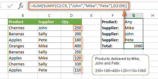
As you see, an array criteria makes the formula much more compact compared to SUMIF + SUMIF, and lets you add as many values as you like in the array.
This approach works with numbers as well as with text values. For instance, if instead of the suppliers' names in column C, you had supplier IDs like 1, 2, 3 etc., then your SUMIF formula would look similar to this:
=SUM(SUMIF(C2:C9, {1,2,3} , D2:D9))
Unlike text values, numbers needn't be enclosed in double quotes in array arguments.
Example 3. SUMPRODUCT & SUMIF
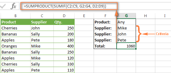
In case, your preferred way is to list the criteria in some cells rather that specify them directly in the formula, you can use SUMIF in conjunction with the SUMPRODUCT function that multiplies components in the given arrays, and returns the sum of those products.
=SUMPRODUCT(SUMIF(C2:C9, G2:G4, D2:D9))
Where G2:G4 are the cells containing your criteria, the suppliers' names in our case, as illustrated in the screenshot below.
But of course, nothing prevents you from listing the values in an array criteria of your SUMIF function if you want to:
=SUMPRODUCT(SUMIF(C2:C9, {"Mike","John","Pete"}, D2:D9))
The result returned by both formulas will be identical to what you see in the screenshot:
Excel SUMIFS with multiple OR criteria
If you want to conditionally sum values in Excel not simply with multiple OR conditions, but with several sets of conditions, you will have to use SUMIFS instead of SUMIF. The formulas will be very similar to what we've just discussed.
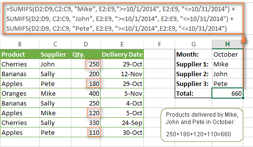
As usual, an example might help to illustrate the point better. In our table of fruit suppliers, let's add the Delivery Date (column E) and find the total quantity delivered by Mike, John and Pete in October.
Example 1. SUMIFS + SUMIFS
The formula produced by this approach includes a lot of repetition and looks cumbersome, but it is easy to understand and, most importantly, it works : )
=SUMIFS(D2:D9,C2:C9, "Mike", E2:E9,">=10/1/2014", E2:E9, "<=10/31/2014") +

SUMIFS(D2:D9, C2:C9, "John", E2:E9, ">=10/1/2014", E2:E9, "<=10/31/2014") +

SUMIFS(D2:D9, C2:C9, "Pete", E2:E9, ">=10/1/2014" ,E2:E9, "<=10/31/2014")
As you see, you write a separate SUMIFS function for each of the suppliers and include two conditions - equal to or greater than Oct-1 (">=10/1/2014",) and less than or equal to Oct 31 ("<=10/31/2014"), and then you sum the results.
Example 2. SUM & SUMIFS with an array argument
I've tried to explain the essence of this approach in the SUMIF example, so now we can simply copy that formula, change the order of arguments (as you remember it is different in SUMIF and SUMIFS) and add additional criteria. The resulting formula is more compact than SUMIFS + SUMIFS:
=SUM(SUMIFS(D2:D9,C2:C9, {"Mike", "John", "Pete"}, E2:E9,">=10/1/2014", E2:E9, "<=10/31/2014"))
The result returned by this formula is exactly the same as you see in the screenshot above.
Example 3. SUMPRODUCT & SUMIFS
As you remember, the SUMPRODUCT approach differs from the previous two in the way that you enter each of your criteria in a separate cell rather that specify them directly in the formula. In case of several criteria sets, the SUMPRODUCT function won't suffice and you will have to employ ISNUMBER and MATCH as well.
So, assuming that the Supplies Names are in cells H1:H3, Start Date is in cell H4 and End Date in cell H5, our SUMPRODUCT formula takes the following shape:
=SUMPRODUCT(--(E2:E9>=H4), --(E2:E9<=H5), --(ISNUMBER(MATCH(C2:C9, H1:H3,0))), D2:D9)
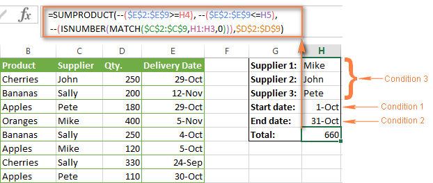
Many people wonder why use double dash (--) in SUMPRODUCT formulas. The point is that Excel SUMPRODUCT ignores all but numeric values, while the comparison operators in our formula return Boolean values (TRUE / FALSE), which are non-numeric. To convert these Boolean values to 1's and 0's, you use the double minus sign, which is technically called the double unary operator. The first unary coerces TRUE/FALSE to -1/0, respectively. The second unary negates the values, i.e. reverses the sign, turning them into +1 and 0, which the SUMPRODUCT function can understand.
I hope the above explanation makes sense. And even if it doesn't, just remember this rule of thumb - use the double unary operator (--) when you are using comparison operators in your SUMPRODUCT formulas.
Using Excel SUM in array formulas
As you remember, Microsoft implemented the SUMIFS function in Excel 2007. If someone still uses Excel 2003, 2000 or earlier, you will have to use a SUM array formula to add values with multiple AND criteria. Naturally, this approach works in modern versions of Excel 2013 - 2007 too, and can be deemed an old-fashioned counterpart of the SUMIFS function.
In the SUMIF formulas discussed above, you have already used array arguments, but an array formula is something different.
Example 1. Sum with multiple AND criteria in Excel 2003 and earlier
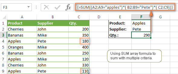
Let's get back to the very first example where we found out a sum of amounts relating to a given fruit and supplier:

As you already know, this task is easily accomplished using an ordinary SUMIFS formula:
=SUMIFS(C2:C9, A2:A9, "apples", B2:B9, "Pete")
And now, let's see how the same task can be fulfilled in early "SUMIFS-free" versions of Excel. First off, you write down all the conditions that should be met in the form of range="condition". In this example, we have two range/condition pairs:
Condition 1: A2:A9="apples"
Condition 2: B2:B9="Pete"
Then, you write a SUM formulas that "multiplies" all of your range/condition pairs, each enclosed in brackets. The last multiplier is the sum range, C2:C9 in our case:
=SUM((A2:A9="apples") * ( B2:B9="Pete") * ( C2:C9))
As illustrated in the screenshot below, the formula perfectly works in the latest Excel 2013 version.
Note. When entering any array formula, you must press Ctrl + Shift + Enter. Once you do this, your formula gets enclosed in {curly braces}, which is a visual indication that an array formula is entered correctly. If you try typing the braces manually, your formula will be converted to a text string, and it won't work.
Example 2. SUM array formulas in modern Excel versions
Even in modern versions of Excel, the power of the SUM function should not be underestimated. The SUM array formula is not simply gymnastics of the mind, but has a practical value, as demonstrated in the following example.
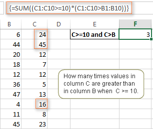
Suppose, you have two columns, B and C, and you need to count how many times column C is greater than column B, when a value in column C is greater or equal to 10. An immediate solution that comes to mind is using the SUM array formula:
=SUM((C1:C10>=10) * (C1:C10>B1:B10))
Don't see any practical application to the above formula? Think about it in another way : )
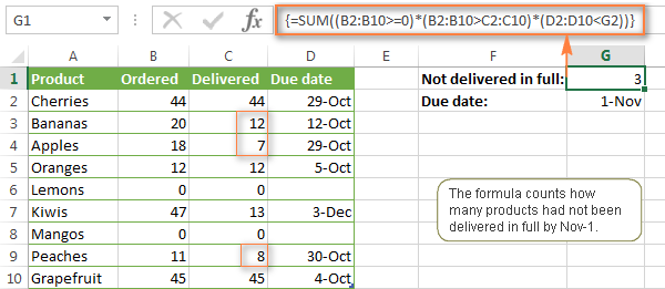
Suppose, you have the orders list like shown in the screenshot below and you want to know how many products have not been delivered in full by a given date. Translated into Excel's language, we have the following conditions:
Condition 1: A value in column B (Ordered items) is greater than 0
Condition 2: A value in column C (Delivered) in less than in column B
Condition 3: A date in column D (Due date) is less than 11/1/2014.
Putting the three range/condition pairs together, you get the following formula:
=SUM((B2:B10>=0)*(B2:B10>C2:C10)*(D2:D10<G2))
Well, the formula examples discussed in this tutorial have only scratched the surface of what Excel SUMIFS and SUMIF functions can really do. But hopefully, they have helped pointing you in the right direction and now you can sum values in your Excel workbooks no matter how many intricate conditions you have to consider.
 by
by
666 comments
I am trying to create a formula that does the following and I cant get the formula to work for all. only one or two of them. but not all of them.
Need a sum for Column J
if Column E = the words Growth or Acquisition
if Column K = the month of July, 2019
So far I have this;
=SUMIFS($J$2:$J$142,$E$2:$E$142,"Growth")+SUMIFS($J$2:$J$142,$E$2:$E$142,"Aquisition")+SUMIFS($J$2:$J$142,$K$2:$K$142,">="&$L$145,$K$2:$K$142,"="&$L$146,$K$2:$K$142,"<="&$M$146))
But its counting the amounts multiple times
I have an updated formula. It is working and not erring out or counting the amounts multiple times however its not catching all amounts.
=SUMIFS($J$2:$J$137,$E$2:$E$137,{"Growth","Acquisition"},$K$2:$K$137,">="&L140,$K$2:$K$137,"<="&M140)
How could I sum two ranges: C20:I20 and C22:I22 using two Criteria ranges: C19:I19 and C21:I21 ... If if any of the cells in the criteria ranges have the criteria "PTO"?
I have tried a few these, but have not been successful:
=SUMIFS(C20:I20, C19:I19,"PTO”) + SUMIFS(C22:I22, C21:I21,”PTO")
=SUMIFS(C20:I20, C19:I19,"PTO”,[C22:I22, C21:I21])
Essentially, I have this working formulas but need to add another Sum_range and Criteria_range to the formula.
Thanks in advance!
I want to make the criteria as dynamic by getting the input from user via slicer. So I tried using sum before sumifs and if I hard code the multiple criteria on the same column it works =sum(sumifs(sum_range, criteria range, {"a","b"}) but if I want to get the input from user via slicer which reference to a cell it doesn't work. =Sum(sumifs(sum_range, criteria range, name_manager).
Name manager to a input which I receive it from user via slicer.
Hi,
can it be used for the Criteria Range the full column for example as I cant get the formula with it. I cant have the exact range as the range is changing from day to day and there is 29000 lines.
No. of months Amount
12 14
20 14
12 9
15 18
25 14
68 18
70 9
Hi Svetlana,
Could you please help me on following,
What is the formula for If i want to calculate total amount in(Column 2) for 12 to 25 months (Column 1) ?
I am greatly appreciate if you could help me on this. Thank you
My congratulations for this excellent article. I already use some criteria for my company.
What I haven't understood is the following: In the formula
=SUMPRODUCT(--(E2:E9>=H4), --(E2:E9<=H5), --(ISNUMBER(MATCH(C2:C9, H1:H3,0))), D2:D9)
the MATCH syntax should say 'Take the value H1:H3, put it to C2:C9, with exact match, eg
--(ISNUMBER(MATCH(H1:H3, C2:C9,0))), D2:D9)
But this gives an error. Why?
Again congratulations for your really excellent article!
I ready type sheet. Some problem formula. Which Lesson 1. Help me
For the second example, if i wanted to return multiple Criteria 1 for example Apples and Oranges Pete has supplied how would I do that?
Hi Chris,
You can do that with one of the below formulas:
=SUM(SUMIFS(C2:C9, A2:A9, {"apples","oranges"}, B2:B9,"pete"))
=SUMIFS(C2:C9, A2:A9,"apples", B2:B9, "pete") + SUMIFS(C2:C9, A2:A9,"oranges", B2:B9, "pete")
Thanks for that it was perfectly. although in some instances i have over 20 criteria and calculating is taking quite a long time. is there a faster way to calculate?
This log has really helped me finding something valuable & usefull, which I may not aware about.
Thanks!!!!
I'm trying to figure out a way to make something like this work but I am unable to do so. Please, will someone help me?
A B C
1 Amounts Condition Result
2 amount 1 if C1=text and B2=empty cell, enter A2; if C1=text and B2=not empty cell, enter A2; if C1=numbers and B2=empty cell enter C1+A2; if C1=numbers and B2=not empty cell enter C1-A2;
3 amount 2 if C2=text and B3=empty cell, enter A3; if C2=text and B3=not empty cell, enter A3; if C2=numbers and B3=empty cell enter C2+A3; if C2=numbers and B3=not empty cell enter C2-A3;
4 amount 2 * if C3=text and B4=empty cell, enter A4; if C3=text and B4=not empty cell, enter A4; if C3=numbers and B4=empty cell enter C3+A4; if C3=numbers and B4=not empty cell enter C3-A4;
5 amount 3 h if C4=text and B5=empty cell, enter A5; if C4=text and B5=not empty cell, enter A5; if C4=numbers and B5=empty cell enter C4+A5; if C4=numbers and B5=not empty cell enter C4-A5;
6 amount 4 if C5=text and B6=empty cell, enter A6; if C5=text and B6=not empty cell, enter A6; if C5=numbers and B6=empty cell enter C5+A6; if C5=numbers and B6=not empty cell enter C5-A6;
7 amount 5 6 if C6=text and B7=empty cell, enter A7; if C6=text and B7=not empty cell, enter A7; if C6=numbers and B7=empty cell enter C6+A7; if C6=numbers and B7=not empty cell enter C6-A7;
So the end result would look and work like this:
A B C
1 Amounts Condition Result
2 10 10
3 15 25
4 20 * 25
5 25 yes 25
6 30 55
7 35 6 55
MR Severity Category Ageing in Days
Bhavnagar NSA Logical Alarm-OMC >3 Days Feedback
Surat SA Physical Alarm - BSS >3 Days OMC Logical
Surat SA Physical Alarm - BSS >3 Days OMC Logical
Ahmedabad SA Physical Alarm - BSS >3 Days RING SPLITTING
Ahmedabad SA Physical Alarm - BSS >3 Days RING SPLITTING
Rajkot NSA Logical Alarm-OMC >3 Days OMC Logical
Ahmedabad SA Physical Alarm - BSS >3 Days TXPL
Ahmedabad SA Physical Alarm - BSS >3 Days TXPL
Baroda SA FAN-Alarm >3 Days FAN FAILURE
Rajkot NSA Logical Alarm-OMC >3 Days wip
Rajkot SA Physical Alarm - BSS >3 Days wip
Ahmedabad NSA Logical Alarm-OMC >3 Days TCTS
Ahmedabad NSA Logical Alarm-OMC >3 Days TCTS
Baroda NSA Physical Alarm - BSS >3 Days VBS_LL services
Baroda NSA Physical Alarm - BSS >3 Days VBS_LL services
Baroda NSA Logical Alarm-OMC >3 Days VBS_LL services
Baroda NSA Physical Alarm - BSS >3 Days VBS_LL services
I am using Sumifs formulea for this attached ment in 2nd Sheet and getting corrected summation pls help to resolved this for 2nd sheet
hi,
i have a list of value is about to 100. i want to know the 6 values which will give a sum of a particular value,
ex:
52636
6326
63699
12563
25699
1236
15693
i want to know 6 values in a above values which give total of 165289.
pls give a solution,
thankyoy
Please help me how to use =sumifs formula to fund the sums more thatn 4 crieteria ranges.
Thanks
Hi,
Can you please help, trying to sum if using multiple criteria including a date range. However it is returning 0.00 value. The date range seems to be the issue as when I remove this the other criteria works. Going around in circles and not sure what I am doing wring.
=SUMIFS('Detail Transaction Listing'!$J:$J,'Detail Transaction Listing'!$D:$D,$B$2,'Detail Transaction Listing'!$A:$A,B15,'Detail Transaction Listing'!$H:$H,">="&Sheet1!$B$5,'Detail Transaction Listing'!$H:$H,"
Sheet 1 B5 & C5 is the criteria field.
Really appreciate your help/
I hoped to have finally found the solution, but it regrettably failed.
{=SUM(($B$38:$B$275=B27)*($C$38:$C$275=C27)*($D$38:$D$275=D27)*($H$38:$H$275))}
In this formula B27, C27 and D27 are the criteria. It works well, ONLY when all criteria cells (B27, C27 and D27) are populated
I was hoping that if one or two of the criteria cells is empty, it would still add $H$38:$H$275 based on whatever criteria (B27 and/or C27 and/or D27) is in place. Instead, the result I'm getting is 0 if one of the criteria is empty.
Any ideas how to solve this?
Lot of thanks to to you. I got the perfect formula at the right time. It saves me lots of time. Great.
=SUMIFS(H2:H1000, D2:D1000,"vehari", G2:G1000, "short")
I want to calculate a range...when two conditions are ture..
But this formula is not working.
Kindly help.
How can I get a count of the number of rows returned using the sumifs function?
My current function is
=SUMIFS $B$2:$B$105,$C$2:$C$105,O111,$D$2:$D$105,O115,$E$2:$E$105,O113)
and I would like to know how many rows were returned to get my total that was returned with the sumifs function.
Thanks,
Matt
This tutorial was a massive help!
Easy to understand and follow, and it works!:)
Thanks so much for providing this for the public!
Hi,I need SUMIFS formula with multiple columns reference.column1-type, column2-length adress, column3- lenghcount. now need total count value with each length adress(column2)
Hi, I am trying to add sum of all outstanding payment of each customer in their respective cell who has crossed the due date but having difficulty in implementing as both criteria has to be checked customer name and the date of supply.
can someone please help
Hi, I am trying to add sum of all outstanding payment of each customer in their respective cell who has crossed the due date but having difficulty in implementing as both criteria has to be checked customer name and the date of supply.
can some please help
Sorry people, read cell A2 as follows
=sumif(criteria range,"Apple",sum range)
Hey people can you tell us how to use sumif for the following;
Criteria 1 - Apple
Criteria 2 -Orange
Criteria 3 -Lemon
Criteria 4 -Pineapple
we want to use sum if to total the sum of "Apples" And all others in s single cell.
eg:
In Cell A1
=sumif(criteria range,"Apple",sum range)
In Cell A2
=sumif(criteria range,"Apple",sum range)
this above formula is not working??? to be specific it sometimes work
also tell us can we apply this formula across sheets in the same excel work book?
awaiting your wise response....
I am trying to make work easier for my team by building a formula that adds up data based on two criteria: The month (this is okay). Each month has for to five weeks. I want the formula to add data in each months for all weeks in the month but up to the current week. I did the formula below. It however appears that Excel does not recognise the last argument below which uses reference to a cell:
=SUMIFS('Weekly targets'!$F$14:$BE$14,'Weekly targets'!$F$1:$BE$1,'Summary by Product'!$E$3,'Weekly targets'!$F$3:$BE$3,"<=$C$4")
Hi,
I need help to put this note in this formula.
=IF(AT1350=400000,0,IF(AT1350<=800000,1000,IF(AT1350<=1200000,2000,IF(AT1350<=2400000,(AT1350-1200000)*5%,IF(AT13504800000,(AT1350-4800000)*15%+(300000)))))))
Note: { Provided that where the taxable income exceeds Rs. 800,000/- the Minimum tax payable shall be Rs. 2,000/-
Hello everyone,
Getting to grips with SUM and SUMIF and have been working on a particular problem using:
=SUM(IF(K10="",O10-P10),IF(K10="PGTA3",O10-(P10/2)))
For this means if "PGTA3" is shown in cell K10 then divide P10 by 2 and subtract the result from O10. However, in the cell K10 I would like this to not be limited to "PGTA3" but anything that includes "PGTA" or "GRP" within the cell.
Essentially O10 is a room size, P10 is a number of students but if ""PGTA or "GRP" is in cell K10 that means there is a second group in another row and the number of students present in the room would be divided in half. Cell K10 could say "PGTA12, "PGTA2", "PGTA3", "GRP1", "GRP2" or a combination of PGTA fields (like "PGTA1,PGTA1" or something like ",PGTA1". The presence of a comma is of no interest to me; if a comma were in a cell alone (it could happen) I want that ignored so I don't think a pure wildcard would work (ie if ANY text in cell K10, divide P10 in half). "PGTA*" and "*" and "*PGTA*" doesn't seem to work anyway and doesn't allow for "GRP". Any help very gratefully received! I aced indexing and array formulas this morning so I'm sure I can ace this too. :)
=SUMIFS('Priority & Standard Cost'!$AJ:$AJ,'Priority & Standard Cost'!$B:$B,Sheet3!B3,'Priority & Standard Cost'!$M:$M,">=04-01-2017",'Priority & Standard Cost'!$M:$M,"='Contract Details'!E3",'Priority & Standard Cost'!$M:$M,"<='Contract Details'!F3")
What is the difference in both formulas.
I have just changed the date from cell in which date is mentioned in same format....but result is 0....Why?
This is my formula:
=SUMIF($C$10:$C$30,"*" & $C$7 &"*",D10:D30)
C7=1 just one number, referring to a shift. So it could be 2 or 3.
D Column = Are just values
Any suggestions.
Last formula solved my problem, Tons of thanks.
What expression do I need to use, to do the following for +100 different criteria, that counts up all quantities in the different criteria's.
=SUM(SUMIF(B2:B152, {"Malus"}, D2:D152))
=SUM(SUMIF(B2:B152, {"Pyrus"}, D2:D152))
to display on the worksheet
Malus 25
Pyrus 36
etc etc for +100 different criteria
Its looking more like I am going to have to use VB code
one more time:
=SUMIFS(ItemizedExpenses[Check Amount], ItemizedExpenses[G/L Code], MonthlyExpensesSummary[@[G/L Code]], ItemizedExpenses[Invoice Date],">=07/01/2018”, “= 07/01/2018”, “<=07/31/2018”)
I am having problems with my SUMIFS. I need to bring the Invoice Amount from two different worksheets over to my main sheet, but I only want them if they match my GL Code and my Monthly Date.
=SUMIFS(ItemizedExpenses[Check Amount], ItemizedExpenses[G/L Code], MonthlyExpensesSummary[@[G/L Code]], ItemizedExpenses[Invoice Date],">=07/01/2018”, “=07/01/2018”, “<=07/31/2018”)
-or-
=SUMIFS(ItemizedExpenses[Check Amount], ItemizedExpenses[G/L Code], MonthlyExpensesSummary[@[G/L Code]], ItemizedExpenses[Invoice Date], MonthlyExpensesSummary[July])
+SUMIFS(Other[Check Amount], Other[G/L Code], MonthlyExpensesSummary[@[G/L Code]], Other[InvoiceDate],[July])
But, neither one work. The top one I can at least get in without error, but doesn't give me results.
Can you help??
Thanks for any assistance,
Tracey
That first one has a typo - it is actually like this:
=SUMIFS(ItemizedExpenses[Check Amount], ItemizedExpenses[G/L Code], MonthlyExpensesSummary[@[G/L Code]], ItemizedExpenses[Invoice Date],">=07/01/2018”, “= 07/01/2018”, “<=07/31/2018”)
Hello,
I am doing multiple calculation and cannot make correct combination of formulas for the following example:
Column1 Column2
4 x
4 x
5
6 x
6 x
7
7
7
I need formula that will conunt criteria from first column without repetition and only for fow that has mark "X" in second column.
For count of first column I used following formula =SUM(IF(FREQUENCY(...), but I cannot cmbinate it with IF second column has "X".
Thanks in advance
Savo
How to calculate Total sales of Google and Costco customer in North East region???
Date Region Sales Rep Customer Product COGS Sales
6/16/2006 NorthEast Jon Google QJV Item $1,835.90 $3,165.34
6/15/2006 NorthEast Jon Amazon.com ZET Item $6,971.50 $9,295.33
6/15/2006 SouthEast Chin Amazon.com ZON Item $5,406.27 $9,163.17
6/15/2006 SouthEast Chin Solar and Wind Inc. JFA Item $736.25 $836.65
6/14/2006 NorthEast Jeri Costco ZET Item $2,065.11 $4,589.14
6/14/2006 NorthEast Troung Sherman Williams LZB Item $2,553.28 $3,754.82
6/14/2006 NorthEast Steven Peet's Coffee EJL Item $2,315.43 $3,405.05
Good day
If you could please advise.
I am trying to do a sumifs using three criteria, but the formula only allows me to add two criteria for evaluation?
Is there a version of excel that allows this, or is there a combination formula that I could use?
Thanking you in advance.
Thank you! Much appreciated help.
{=sum((F:F="")*(A:A<20)*(B:B))}
F = Name , A = Value , B = Value
I use this formula when I want to know the value which is under 20). This is fine. All I wanna know is how can I calculate the value which between 20 to 50. Please help me out.
Svetlana Cheusheva, you are fantastic. This was quite a piece of valuable information. Thanks a lot, you made my day.
I have a person information spreadsheet with about 2000 rows. I need a formula that will total the 'Sex' and 'Race' columns for the gender and race details. Ex. White Males = ?
Black Males = ? White Females = ?. The single criteria in the 'Sex' column will be either M or F. The 'Race' criteria will be a single identifier for the race. This seems to be a common problem but I cannot make it work. Thanks for any help.
Hello, David:
With that many rows of data I would use a Pivot Table.
QUESTION
Rubber Material Qty1 Cushion Gum Qty2
LL215-128 11.5 CUS GUM 225 MM-EB 1.3
LL215-128 11 CUS GUM 200 MM 1.3
60-62-18-P-Mtk 2.5 CUS GUM 200 MM 1.3
NH165-103 3/4 6.6 CUS GUM 165 MM 0.6
FR175-119 6.8 CUS GUM 165 MM 0.7
NH165-103 3/4 6.6 CUS GUM 165 MM 0.7
FR175-119 6.8 CUS GUM 165 MM 0.8
NH165-103 3/4 6.7 CUS GUM 165 MM 0.6
FR175-119 6.8 CUS GUM 165 MM 0.7
NH165-103 3/4 6.8 CUS GUM 165 MM 0.6
NH165-103 3/4 6.7 CUS GUM 165 MM 0.6
LG-215-128-VT 10.2 CUS GUM 225 MM-EB 1.5
LG-215-128-VT 10.1 CUS GUM 225 MM-EB 1.4
LG-215-128-VT 10.1 CUS GUM 225 MM-EB 1.5
SM 220-128 12.4 CUS GUM 225 MM-EB 1.4
SM 240-130 12.4 CUS GUM 225 MM-EB 1.5
SM 230-130 12.7 CUS GUM 225 MM-EB 1.5
SM 230-130 12.7 CUS GUM 215 MM-EB 1.5
SM 220-130 12.4 CUS GUM 225 MM-EB 1.4
SM 230-130 12.8 CUS GUM 215 MM-EB 1.4
SM 230-130 12.7 CUS GUM 225 MM-EB 1.4
SM 230-130 12.7 CUS GUM 215 MM-EB 1.5
Rl 210-127 11.4 CUS GUM 200 MM 1.4
Rl 210-127 11.4 CUS GUM 200 MM 1.5
RESULT: I WANT TO KNOW SUM OF MATERIAL USED WITH HELP OF SUM-IF / OTHERWISE ANY OTHER FORMULA IS THERE.
MATERIAL
60-62-18-P-Mtk
CUS GUM 165 MM
CUS GUM 200 MM
CUS GUM 215 MM-EB
CUS GUM 225 MM-EB
FR175-119
LG-215-128-VT
LL215-128
NH165-103 3/4
Rl 210-127
SM 220-128
SM 220-130
SM 230-130
SM 240-130
i need sumifs function -- my company loaded flour every day 14 trucks for different companeis . so i need each company howmany ton per day? so please help me
Hello,
I am doing a multiple criteria SUMIFS but with one range I'd like it to be an OR. (The works great for multiple if there are only one or two NOTS, but there are several 'not wanted' and only 2 wanted.)
I can do a SUMIFS + SUMIFS but the braces option do not seem to work for a cell reference being used for the criteria:
working:
=SUMIFS($K$4:$K$503,$H$4:$H$503,"=" & $AA45,$F$4:$F$503,"Renewal",$L$4:$L$503,"="&DropDowns!$A$28 ) + SUMIFS($K$4:$K$503,$H$4:$H$503,"=" & $AA45,$F$4:$F$503,"Renewal",$L$4:$L$503,"="&DropDowns!$A$27 )
but want to do something like this (since all other criteria is the same)
... $H$4:$H$503,"=" & $AA45,$F$4:$F$503,"Renewal"
============================================================
=SUMIFS($K$4:$K$503,$H$4:$H$503,"=" & $AA45,$F$4:$F$503,"Renewal",$L$4:$L$503,{"="&DropDowns!$A$28,"="&DropDowns!$A$27} )
is it placement? Does the 'or' criteria need to be first? (the Or function does not work here)
$L$4:$L$503,{"="&DropDowns!$A$28,"="&DropDowns!$A$27}
Is there another sequence for the braces? {"="&DropDowns!$A$28,"="&DropDowns!$A$27}
The weird "="&cell is the only way my system will allow the criteria in that cell to be used maybe since it is a text.
Thank you for any insight.
excel formula for 25 mg*2=50 mg
I would like to sum the Expected Payment column if the date in the Payment Due Date column is a date in 2018. I have tried both sumif and sumproduct, however, I believe that since the columns I am referencing are formulas which generate a $, date, or blank, it is not working.
K13:K36=Expected Payment (is a formula that generates a $ or blank) L13:L36=Payment Due Date (is a formula that generates a date of blank)
If someone has an answer for this, it would be greatly appreciated! :)
Hi Svetlana Cheusheva,
Hope you are doing good.....
I have couple of question on Sum formula.
Sum it to total
Sumif is to total with one condition/Criteria
Sumifs is to total with one or more condition/criteria that to if all condition/criteria satisfy only then only it display the results that is output. my question it should give the output or result even if any one condition/criteria satisfy also.
Thanks in advance
Mahaboob
Hello, please can someone help me?
I have 2 sheets, one with the current sales by location and the other sheet exactly the same but without figures. I basically need to model it for different scenarios.
This is how it works in my head but not in reality.
=IF(Scenarios!B1="1",SUMIF('Project Sales month only'!C:C,Scenarios!C3,'Project Sales month only'!I:I*2))
I have 3 different scenarios so will need to add the other 2 if statements on but please can someone help me?
Thanks in advance
Hi, I am trying to SUMIF the following:
Channel, Product and Price
Under channel column I have different criteria: agent, google, organic, etc.
Under product: 5 different products/criteria
Under price: products actual prices that I want to get it summed accordingly.
i.e.: Channel range. I want to sum all google leads for the various products.
for Google sales, MBA products only, Google sales, Postgraduate Certificates, etc.
This is what I am doing but it is not summing correctly.
=SUMIFS(J2:J40,$B$2:$B$40, "google",$F$2:$F$40,"PGC")+SUMIFS(J2:J40,$B$2:$B$40,"facebook",$F$2:$F$40,"PGC")+SUMIFS(J2:J40,$B$2:$B$40,"organic",$F$2:$F$40,"PGC")+SUMIFS(J2:J40,$B$2:$B$40, "affiliate",$F$2:$F$40,"PGC")+SUMIFS(J2:J40,$B$2:$B$40, "alumni",$F$2:$F$40,"PGC")+SUMIFS(J2:J40,$B$2:$B$40, "referral",$F$2:$F$40,"PGC")
In the end I want to find out how much sales we got from google for a particular product.
Can you help, please?
thanks,
Guiherme
Guiherme, Would it work if you put the absolute$ reference on the J2:J40 AND put a space before and after each of the + symbols ?
was >>>SUMIFS(J2:J40,$B$2:$B$40, "google",$F$2:$F$40,"PGC")+SUMIFS(J2:J40...
try>>> SUMIFS($J$2:$J$40,$B$2:$B$40,"google",$F$2:$F$40,"PGC") + SUMIFS($J$2:$J$40...
a space before and after the + symbol may help the formula work consistently.
Hope something works out for you.
Ruth
Thanks for give me the strong understanding and useful knowledge
1.5hrs+0.3hrs=?hrs how to calculate time in this form
Hello,
If I understand your task correctly, please try the following formula:
=TEXT((1.5+0.3)/24,"hh:mm")
Hope this will help.