The VLOOKUP function is the most popular lookup and reference function in Excel. It is also one of the trickiest and the dreaded #N/A error message can be a common sight.
This article will look at the 6 most common reasons why your VLOOKUP is not working.
You Need an Exact Match
The last argument of the VLOOKUP function, known as range_lookup, asks if you would like an approximate or an exact match.
In most cases people are looking for a particular product, order, employee or customer and therefore require an exact match. When looking for a unique value, FALSE should be entered for the range_lookup argument.
This argument is optional, but if left empty, the TRUE value is used. The TRUE value relies on your data being sorted in ascending order to work.
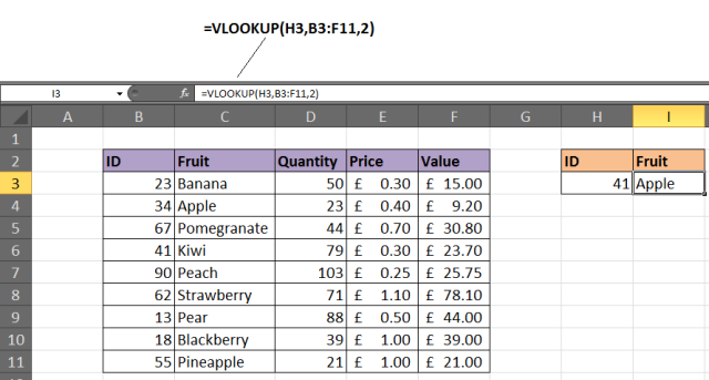
The image below shows a VLOOKUP with the range_lookup argument omitted, and the incorrect value being returned.
Solution
If looking for a unique value, enter FALSE for the last argument. The VLOOKUP above should be entered as =VLOOKUP(H3,B3:F11,2,FALSE).
Lock the Table Reference
Maybe you are looking to use multiple VLOOKUPs to return different information about a record. If you are planning to copy your VLOOKUP to multiple cells, you will need to lock your table.
The image below shows a VLOOKUP entered incorrectly. The wrong cell ranges are being referenced for the lookup_value and table array.

Solution
The table that the VLOOKUP function uses to look for and return information from is known as the table_array. This will need to be referenced absolutely to copy your VLOOKUP.
Click on the references within the formula and press the F4 key on the keyboard to change the reference from relative to absolute. The formula should be entered as =VLOOKUP($H$3,$B$3:$F$11,4,FALSE).
In this example both the lookup_value and table_array references were made absolute. Typically it may be just the table_array that needs locking.
A Column Has Been Inserted
The column index number, or col_index_num, is used by the VLOOKUP function to enter what information to return about a record.
Because this is entered as an index number, it is not very durable. If a new column is inserted into the table, it could stop your VLOOKUP from working. The image below shows such a scenario.
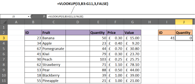
The quantity was in column 3, but after a new column was inserted it became column 4. However the VLOOKUP has not automatically updated.
Solution 1
One solution might be to protect the worksheet so that users cannot insert columns. If users will need to be able to do this, then it is not a viable solution.
Solution 2
Another option would be to insert the MATCH function into the col_index_num argument of VLOOKUP.
The MATCH function can be used to look for and return the required column number. This makes the col_index_num dynamic so inserted columns will no longer affect the VLOOKUP.
The formula below could be entered in this example to prevent the problem demonstrated above.

The Table has got Bigger
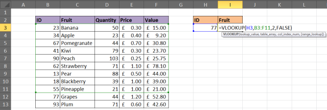
As more rows are added to the table, the VLOOKUP may need to be updated to ensure that these extra rows are included. The image below shows a VLOOKUP that does not check the entire table for the item of fruit.
Solution
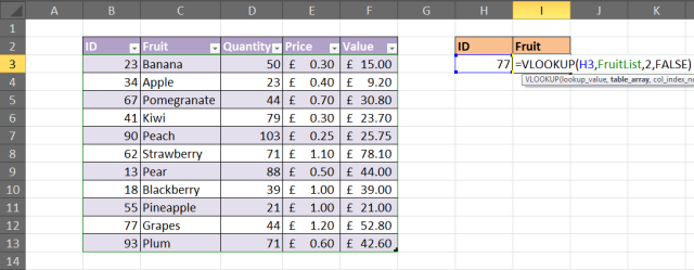
Consider formatting the range as a table (Excel 2007+), or as a dynamic range name. These techniques will ensure that your VLOOKUP function will always be checking the entire table.
To format the range as a table, select the range of cells you want to use for the table_array and click Home > Format as Table and select a style from the gallery. Click the Design tab under Table Tools and change the table name in the box provided.
The VLOOKUP below shows a table named FruitList being used.
VLOOKUP Cannot Look to its Left
A limitation of the VLOOKUP function is that it cannot look to its left. It will look down the leftmost column of a table and return information from the right.
Solution
The solution to this involves not using VLOOKUP at all. Using a combination of the INDEX and MATCH functions of Excel is a common alternative to VLOOKUP. It is far more versatile.
The example below shows it being used to return information to the left of the column you are looking in.
Your Table Contains Duplicates
The VLOOKUP function can only return one record. It will return the first record that matches the value you looked for.
If your table contains duplicates then VLOOKUP will not be up to the task.
Solution 1
Should your list have duplicates? If not consider removing them. A quick way to do this is to select the table and click the Removes Duplicates button on the Data tab.
Check out the AbleBits Duplicate Remover for a more complete tool for handling duplicates in your Excel tables.
Solution 2
Ok, so your list should have duplicates. In this case a VLOOKUP is not what you need. A PivotTable would be perfect to select a value and list the results instead.
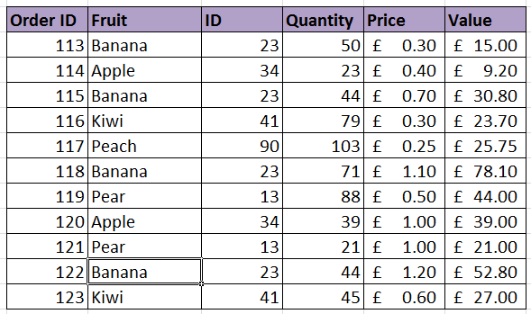
The table below is a list of orders. Let's say you want to return all the orders for a particular fruit.
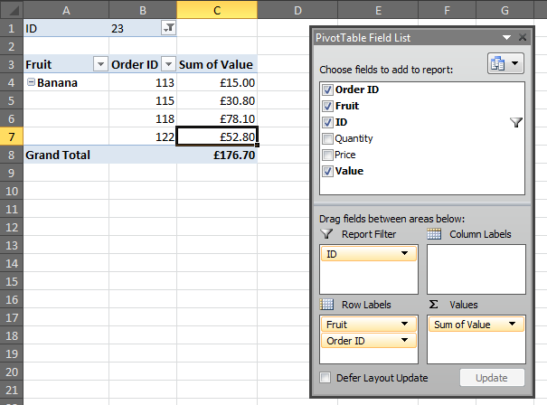
A PivotTable has been used to enable a user to select a Fruit ID from the report filter and a list of all the orders appears.
Trouble Free VLOOKUPs
This article demonstrated a solution to the 6 most common reasons a VLOOKUP function is not working. Armed with this information you should enjoy a less troublesome future with this awesome Excel function.
About the Author
Alan Murray is an IT Trainer and the founder of Computergaga. He offers online training and the latest tips and tricks in Excel, Word, PowerPoint and Project.
 by
by 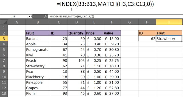
223 comments
another tip: if you're looking up numbers, make sure they are not 'numbers formatted as text.' They'll break the formula.
Thanks Bill.
Yes to add to that... the formatting of the lookup value and the first column of the table array must match. Whether they both be numbers, or both be numbers formatted as text, they must be the same.
I have tried all the solutions the article mentioned, still failed then I tried this, always start the looking table with the value you are looking for in the first column e.g. VLOOKUP(sheet1!A2, sheet2!$C$2:$E$84, 1, FALSE). That is you are looking for value in column C in sheet2 that matches value in column A in sheet1. It is magic! to solve a problem of VLOOKUP that happens when we copy data from different data sources.
Thanks for the tip JimmyNZ.
Yes VLOOKUP will only return the first match. You can use a PivotTable to perform actions like show all invoice # for a particular aircraft.
Otherwise if you wish to populate a bunch of cells with this info then you are looking for a macro probably.
Hi! I worked in airline company and one task I have is to matched the invoice # to a particular aircraft
I used vlookup but it will only return the first match. Sometime an aircraft comes multiple times in a month. How do I solve this?
Yes VLOOKUP will only return the first match. You can use a PivotTable to perform actions like show all invoice # for a particular aircraft.
Otherwise if you wish to populate a bunch of cells with this info then you are looking for a macro probably.
Thank you guys, great page!
Thank you very much!! It worked. I forgot to lock my table.
columns values same but rows values change how can use vlookup formula
E.g.
Same Change Value
Name AAAA BBBB CCCC DDDD
A 15 12 16 22
B 45 26 33 99
C 88 33 78 98
B 22 34 56 37
Hi,
I’m trying to use VLOOKUP to look up values with a combination of FS500000, 1000000, F500000. The VLOOKUP is finding combination FS500000 and F500000, however fields with 1000000 are showing the #NA error.
The cells are formatted as general (also tried switching to text), i've removed "hidden" fields and inserted TRIM within the formula, but still no luck.
It’s just a simple VLOOKUP formula of =VLOOKUP(A9,Sheet2!A1:K10000,6,FALSE)
Any help would be appreciated.
Thanks.
Hi Simon,
I did suspect this would be due to the formatting. General is not adequate, Excel will still view 1000000 as a number.
Formatting as text is good. Just ensure the lookup value and the first column of the table array are the same format. So both need to be text.
Hope it works out.
Alan
I keep receiving a #REF! error when using a VLOOKUP between two workbooks on a network share.
If I have the VLOOKUP workbook open (showing the #REF! errors) and then I open up the workbook that contains the table array - then the #REF! errors disappear and the cells contain the correct data. It seems as if I must have the source workbook open in order for the link between the two to function correctly. Do you have any suggestions that I could try?
i make a table using vlookup but its not working properly.
in same row some times show result okay some times not okay. how to resolve. pls help
I can't really explain without more information. Maybe check the typing of the entries.
You say it works for some and not others. Sounds like a mis-type on those entries not working. Or maybe the second reason above.
I am unable to do vlookup between 2 google sheets. 2 sheets are not getting linked.
I do not use Google Sheets but am under the impression it works in a similar way. I would re-check the VLOOKUP for potential mistake.
can someone please help urgently. i am trying to find the status for the sales but it is only working for the price. pleasee help!!! i don't know what to do!!
USE FUNCTION
Vlookup IF
Brand Products Quantity Price Sales Status Tax
Samsung Projector 15 $1,500.00 $22,500.00 Poor
HP L Printer 20 $1,200.00 $24,000.00 Poor
APPLE Mac/Air 5 $2,200.00 $11,000.00 Poor
Samsung Laptop 10 $1,600.00 $16,000.00 Poor
HP Camera 25 $800.00 $20,000.00 Poor
Samsung Galaxy tab 12 $1,200.00 $14,400.00 Poor
ACER Netbook 18 $900.00 $16,200.00 Poor
DELL DUO/Laptop 13 $2,500.00 $32,500.00 Poor
APPLE Ipad 4 16 $1,400.00 $22,400.00 Poor
TOTAL =>
STATUS more than $30,000.00 Excellent
more than $25,000.00 Good
more than $20,000.00 Average
more than $15,000.00 Trial
less than $15,000.00 Poor
TAX more than $30,000.00 25% Of SALES
more than $25,000.00 20%
more than $20,000.00 15%
more than $15,000.00 10%
less than $15,000.00 5%
Alan,Thank you very much!!!!!
Another issue can be "unknown characters" instead of spaces being used. I was looking at a file with 2 sets of data that looked the same, but they were extracted by different means from a database, and on one set of data, spaces were not spaces but some other character. Found it by checking if 2 items that look identical were actually identical (they weren't, according to Excel), and the only possible characters that could be different were those I couldn't see, i.e. spaces.
Yes sometimes data needs to be cleansed after importing from a database before formulas such as VLOOKUP can be run.
Text functions such as SUBSTITUTE and TRIM are great for this sort of tasks. The Find & Replace and Power Query tools are also brilliant for cleansing data.
i want to use vlookup function my data have duplicate value but i don't want to remove it ,so i want use vlookup function but it gave me the first value of duplicate value i want to find the second value that belong to duplicate please help me
Hi Farid,
Check out this video - https://youtu.be/QAZ3L6xbNJc
It shows how to use VLOOKUP to return the last match if there are duplicates. You can adapt this easily for the 2nd match though.
Alan
Hi Alan
I'm doing a VLOOKUP which I do every month to put dates next to asset ID numbers. My LOOKUP results are exactly the same for every ID number when i copy down my formula. So the results for the first row are correct but the rest are wrong as they're the same as the first.
Hi Mel,
It sounds like your lookup_value is absolute so is not changing when you copy the formula.
You might need to remove the dollar signs from the first part of your VLOOKUP.
Alan
While selecting rows and col in vlookup formula (the area where to search) the row col reference (eg. 8RX4C) is not displaying, It is getting difficult to count manually for larger tables.
Please help me on this issue
Thanks in advance
I'm struggling a little with the question but I think you are asking about entering the col index num when using a big table.
In such an example the MATCH function can be used to look along the header row and locate the column number for you. This is done in a similar way to the 5th example of this tutorial and in the link below.
http://www.computergaga.com/tips/lookup_formulas/two_way_lookup_using_index_and_match.html
Hello, Please help me understand why my vlookup formula stops working after 10 matches. My formula is very simple: =VLOOKUP(A7,'compiled responses'!B7:C804,1) my data is very simple: column "a" has numbers, column "b" has numbers
col A col B
404523 404523
447135 447135
447350 447135 this is where the formula stops working as it returns the incorrect value and then the values become N/A.
I have checked the data is has no blanks, both columns are general input.
I look forward to your assistance.
Kindly,
DH
I think your VLOOKUP by the sound of it is comparing columns A and B. And in this case it is stopping at that point because it is not a match i.e. 447350 is not equal to 447135.
number could also be stored as text
Very true. The formatting of the values stored and the one searched for must be consistent.
Hi. Thanks for your reply. Unfortunately, it's still not working, even with all values consistent. Totally baffled!
Hi - VLOOKUP is working fine for me apart from only returning the first letter, i.e returning only 'J' instead of John. Any ideas?
Not a clue. VLOOKUP will return all of the content from the cell, so as long as the full name is in there it will work.
HI
I want to use VLOOKUP with two diffrent spreadsheet which containt no match value on both, in that case is it possible to apply VLOOKUP in this manner??
It is possible to apply a VLOOKUP to two different spreadsheets. Ensure both workbooks are open when you write the VLOOKUP.
Not sure what you mean by the contain no match on both, but VLOOKUP can help check for matches so sounds like it would work.
Hi Alan...
Do you have any idea why my VLOOKUP stopped refreshing automatically for ALL my spreadsheets. In your example, when I change I3, I actually have to click into the formula in J3 and hit enter for it to pull the refreshed value.
Hi Carlo,
I think the cells containing the VLOOKUP's are formatted as text. I would select the cells and check the formatting on the Home tab.
It may also be that you have manual calculation switched on. Click the Formulas tab and then Calculation Options.
Alan
Why VLOOKUP with "TRUE" condition is not working on dates?
It should work with dates no problem. Ensure the table is sorted in earliest to latest by the date.
Thank you, the 'VLOOKUP cannot look to its left' was my pain was my issue. Totally unintuitive
VLOOKUP Cannot Look to its Left was my issue.. thanks!
Thank you Alan, you helped me with The Table has got Bigger.
Thank you! My error wasn't any of these, but it was good to be encouraged to look through everything piece by piece. Turns out I had the initial column and the lookup_value formatted differently--one was Number and the other wasn't (somehow...) So, another goofy mistake, but maybe it will help someone.
Why does my vlookup give the same answer?
Hi,
My table has duplicates in lookup cell, but the value against it is unique, what should I do if I want all the values populated?
e.g
Column A Column B
Banana USA
Watermelon Brazil
Banana Columbia
Now if I want both USA and Columbia in how should I get it, as vlookup only gives USA?
@Gautam Lapsiya Yes the VLOOKUP will only return the first answer.
An option is to use a PivotTable like in the last example.
Alan
Thanks Alan
Watched the YouTube video and it was brilliant instruction!
Saved me loads of time and frustration.
Thanks so much.
You might be able to concatenate a string. Wrap the * in "" to indicate that you want to refer to that character literally and not as a wildcard.
Otherwise you might be able to use the EXACT function with INDEX and MATCH instead of VLOOKUP. Information on this can be found below.
http://www.computergaga.com/tips/lookup_formulas/case_sensitive_lookup.html
I have not tested this, but think it should work. This function does what its name suggest and ensure the strings match.
That might be. My ERP system only allows * as special characters so all my item number data exports have * in them. Do you know of a way to prevent this?
I am trying to write a VLookup formula to bring on hand data into a sheet that details sales volume. My formula is:: =VLOOKUP(A2,AA$2:AB$100,2,FALSE)
Item B1007080SHF3MDO2BS***GG is not present on the target range; Item B1007080SHF3MDO2BSR**GG is there, with a required response value of 409.
When I apply the VLookup to both fields, I get the value of 409 for BOTH, so the 'exact value' part of the formuala does not seem to be working. I have both lists sorted A-Z. It does not seem to matter if I format both columns as text or numbers, same issue (the full data set column does have values that are numbers only & alpha-numeric in both the search criteria and the target range).
It looks like the VLOOKUP is using the ** characters as a wildcard.
Hard to say exactly without seeing the file. Check that there is definitely a match, so no spaces after the number. And also check the formatting of both the lookup_value and on the table_array to check they are the same.
i am doing a very simple lookup and I am getting the #n/a. Trying to pull a number into my master. The first column on both is my ref. the formula is =vlookup(A2,PLANC,2,false). Very very simple. I checked to make sure there was a match and there was and no duplicates were found. Help!
I was having the same issue and just figured it out! (getting #N/A when I know there's an exact match)
If you see the green triangle on the cell, hover over the yellow exclamation point "Number stored as text". From the dropdown select "Convert to Number" and it will fix it immediately. Good luck!
Well done, Jen.
Yes, the two values must be the same format.
Thanks for sharing. I had some hidden columns so my VLOOKUP was not working! Fixed it after readong Point 3. on your list.
VLOOKUP won't be able to. It will only return the first name from the sheet.
You will need more than 1 VLOOKUP. Or a macro would be needed for multiple occurrances of a name.
can any help me put
i had a sheet of name of the employs and their working hours, here the problem is in my sheet i had two names similar...(EX: mahesh as two time in the sheet )
when i use vlookup in the table for my sheet i am not getting the second name
how can i get the second name in the sheet........by using vlookup
Thank you, thank you, thank you for the manual - automatic guide.
Hi Don,
Having calculation set from manual to automatic is very helpful. Save lots of time.
Thank you very much.
Andy
thank you
Hard to say why without seeing the spreadsheet but would expect there to be an error in the lookup value argument. I would check the reference.
Hopefully someone can help me. My vlookup is returning the correct values in my columns but it returns the same value until it comes across another non-zero value. For example the correct value of row 10 is 259 but it will return 259 for rows 11, 12, and 13. Row 14 will correctly show 864 but then rows 15 and 16 will too.
Has anyone come across this?
thanks,
Have the same issue. VLOOKUP is used only for values in ASCENDING order! Try Index Match combination instead.
thanks a lot for this information
Thanks a lot! very helpful :)
Sometimes the error may be because it has not calculated properly. If you have calculation set to manual rather than automatic, this can also cause an error when using vlookup or index match. Once the worksheet calculation is set to automatic, it works again (set it to automatic by going to the Formulas tab and then Calculation Operations and set to Automatic).
Dan,
THANK YOU!!! Hours wasted, but many more hours saved. The Automatic setting in Calculation Operations did it. Karma credits in the heapful submitted your way.
Thank u Dan.
I was trying to copy formula and wasted hours. ur just one line comment solved my problem in a tick
:)
Thank you so much Dan! This annoying setting has wasted me hours before!
This has saved my hours of hair-pulling ! I have been working with vlookup for a long time now but had not encountered this problem before. Many thanks !
OMG.. thanks so much .. was trying a few times why my excel keep seem to be repeating the same value.
Massive thanks for this tip! I couldn't figure it out!!!
You're welcome, Anna.
when we using vlookup it is show is same number in all colons
Me too is facing a similiar error.
Have you got any solution for this.please let me know
I'm not sure what you need. Do you mean all columns?
You would need a VLOOKUP in each. A formula can only return to one cell.
save the sheet, it will run the lookup
Thank you, it was helpful.
The trapfall of VLOOKUP being not able to "look to right" wasn't known to me before. Very helpful!
Thank you, it was helpful.