The tutorial explains all main features of Excel conditional formatting with examples. You will learn how to do conditional formatting in any version of Excel, efficiently use preset rules or create new ones, edit, copy and clear formatting.
Excel conditional formatting is a really powerful feature when it comes to applying different formats to data that meets certain conditions. It can help you highlight the most important information in your spreadsheets and spot variances of cell values with a quick glance.
Many users, especially beginners, find it intricate and obscure. If you feel intimidated and uncomfortable with this feature, please don't! In fact, conditional formatting in Excel is very straightforward and easy to use, and you will make sure of this in just 5 minutes when you have finished reading this tutorial :)
What is conditional formatting in Excel?
Excel Conditional Formatting is used to apply certain formatting to data that meets one or more conditions. Just like usual cell formatting, it lets you highlight and differentiate your data in various ways by changing cells' fill color, font color, border styles, etc. The difference is that it is more flexible and dynamic - when the data changes, conditional formats get updated automatically to reflect the changes.
Conditional formatting can be applied to individual cells or entire rows based on the value of the formatted cell itself or another cell. To conditionally format your data, you can utilize preset rules such as Color Scales, Data Bars and Icon Sets or create custom rules where you define when and how the selected cells should be highlighted.

Where is conditional formatting in Excel?
In all versions of Excel 2010 through Excel 365, conditional formatting resides in the same place: Home tab > Styles group > Conditional formatting.
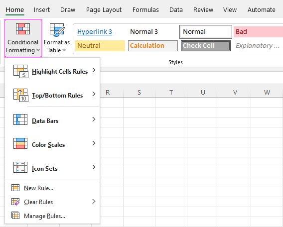
Now that you know where to find conditional formatting in Excel, let's move on and see how you can leverage it in your daily work to make more sense of the project you are currently working on.
For our examples, we will use Excel 365, which seems to be the most popular version these days. However, the options are essentially the same in all Excels, so you won't have any problems with following no matter what version is installed on your computer.
How to use conditional formatting in Excel
To truly leverage the capabilities of conditional format, you need to learn how to utilize various rule types. The good news is that whatever rule you are going to apply, it defines the two key things:
- What cells are covered by the rule.
- What condition should be met.
So, here's how you use Excel conditional formatting:
- In your spreadsheet, select the cells you want to format.
- On the Home tab, in the Styles group, click Conditional Formatting.
- From a set of inbuilt rules, choose the one that suits your purpose.
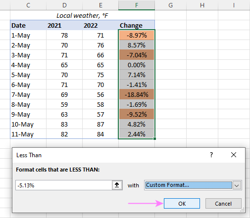
As an example, we are going to highlight values less than 0, so we click Highlight Cells Rules > Less Than…
- In the dialog window that appears, enter the value in the box on the left and choose the desired format from the drop-down list on the right (default is Light Red Fill with Dark Red Text).
When done, Excel will show you a preview of formatted data. If you are happy with the preview, click OK.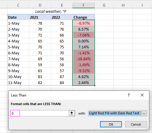
In a similar manner, you can use any other rule type that is more appropriate for your data, such as:
- Greater than or equal to
- Between two values
- Text that contains specific words or characters
- Date occurring in a certain range
- Duplicate values
- Top/bottom N numbers
How to use a preset rule with custom formatting
If none of the predefined formats suits you, you can choose any other colors for cells' background, font or borders. Here's how:
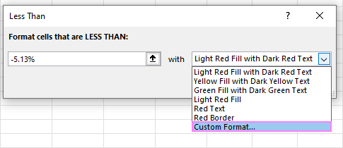
- In the preset rule dialog box, from the drop-down list on the right, pick Custom Format…
- In the Format Cells dialog window, switch between the Font, Border and Fill tabs to choose the desired font style, border style and background color, respectively. As you do this, you will immediately see a preview of the selected format. When done, click OK.
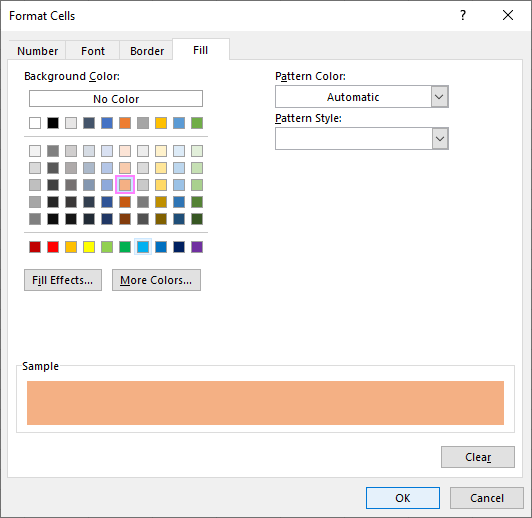
- Click OK one more time to close the previous dialog window and apply the custom formatting of your choice.
Tips:
- If you want more colors than the standard palette provides, click the More Colors… button on the Fill or Font tab.
- If you wish to apply a gradient background color, click the Fill Effects button on the Fill tab and choose the desired options.
How to create a new conditional formatting rule
If none of the preset rules meets your needs, you can create a new one from scratch. To get it done, follow these steps:
- Select the cells to be formatted and click Conditional Formatting > New Rule.

- In the New Formatting Rule dialog box that opens, select the rule type.
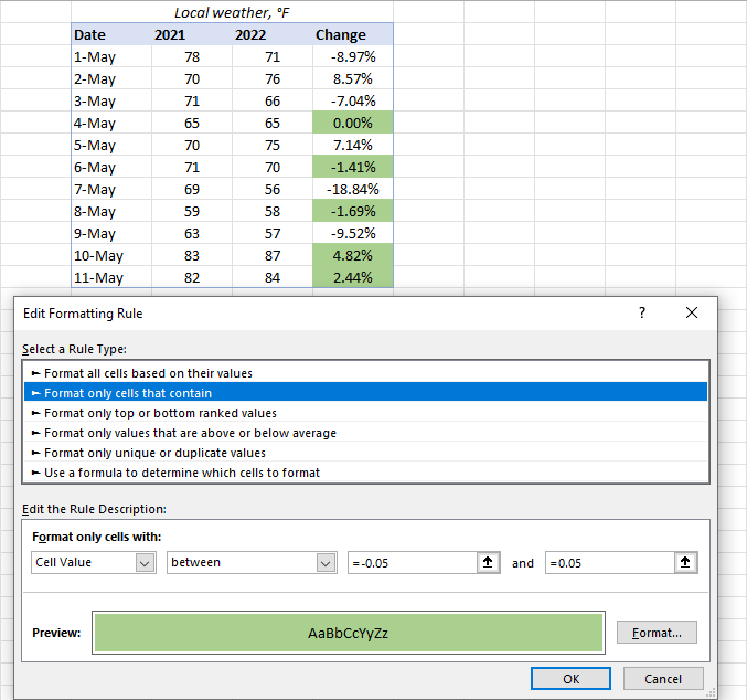
For example, to format cells with percent change less than 5% in either direction, we choose Format only cells that contain, and then configure the rule like shown in the screenshot below: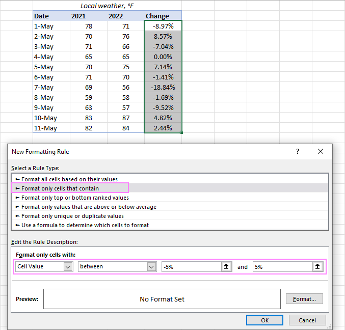
- Click the Format… button, and then choose the Fill or/and Font color you want.
- Click OK twice to close both dialog windows and your conditional formatting is done!
Excel conditional formatting based on another cell
In the previous examples, we highlighted cells based on "hardcoded" values. However, in some cases it makes more sense to base your condition on a value in another cell. The advantage of this approach is that irrespective of how the cell value changes in future, your formatting will adjust automatically to respond to the change.
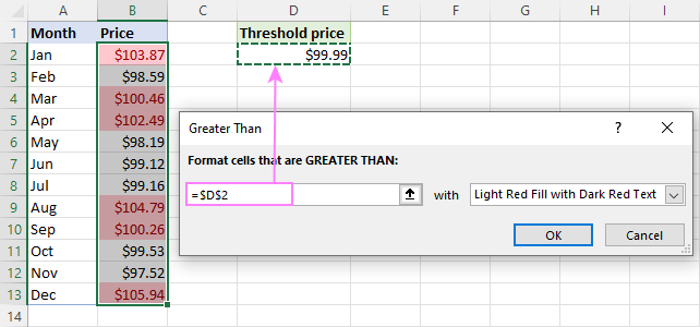
As an example, let's highlight prices in column B that are greater than the threshold price in cell D2. To accomplish this, the steps are:
- Click Conditional formatting> Highlight Cells Rules > Greater Than…
- In the dialog box that pops up, place the cursor in the text box on the left (or click the Collapse Dialog icon), and select cell D2.
- When done, click OK.
As a result, all the prices higher than the value in D2 will get highlighted with the selected color:
That is the simplest case of conditional formatting based on another cell. More complex scenarios may require the use of formulas. And you can find several examples of such formulas along with the step-by-step instructions here:
Apply multiple conditional formatting rules to same cells
When using conditional formats in Excel, you are not limited to only one rule per cell. You can apply as many rules as your business logic requires.
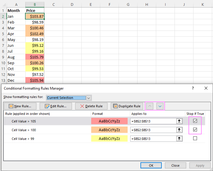
For example, you can create 3 rules to highlight prices higher than $105 in red, higher than $100 in orange, and higher than $99 in yellow. For the rules to work correctly, you need to arrange them in the right order. If the "greater than 99" rule is placed first, then only the yellow formatting will be applied because the other two rules won't have a chance to be triggered - obviously, any number that is higher than 100 or 105 is also higher than 99 :)
To re-arrange the rules, this is what you need to do:
- Select any cell in your dataset covered by the rules.
- Open the Rules Manager by clicking Conditional Formatting > Manage Rules…
- Click the rule that needs to be applied first, and then use the upward arrow to move it to top. Do the same for the second-in-priority rule.
- Select the Stop If True check box next to all but the last rule because you do not want the subsequent rules to be applied when the prior condition is met.
What is Stop if True in Excel conditional formatting?
The Stop If True option in conditional formatting prevents Excel from processing other rules when a condition in the current rule is met. In other words, if two or more rules are set for the same cell and Stop if True is enabled for the first rule, the subsequent rules are disregarded after the first rule is activated.
In the example above, we have already used this option to ignore subsequent rules when the first-in-priority rule applies. That usage is quite evident. And here are another couple of examples where the use of the Stop If True function is not so obvious but extremely helpful:
How to edit Excel conditional formatting rules
To make some changes to an existing rule, proceed in this way:
- Select any cell to which the rule applies and click Conditional Formatting > Manage Rules…
- In the Rules Manager dialog box, click the rule you want to modify, and then click the Edit Rule… button.

- In the Edit Formatting Rule dialog window, make the required changes and click OK to save the edits.
That dialog window looks very similar to the New Formatting Rule dialog box used for creating a new rule, so you won't have any difficulties with it.
Tip. If you don't see the rule you want to edit, then select This Worksheet from the Show formatting rules for drop-down list at the top of the Rules Manager dialog box. This will display the list of all the rules in your worksheet.
How to copy Excel conditional formatting
To apply a conditional format you've created earlier to other data, you won't need to re-create a similar rule from scratch. Simply use Format Painter to copy the existing conditional formatting rule(s) to another data set. Here's how:
- Click any cell with the formatting you want to copy.
- Click Home > Format Painter. This will change the mouse pointer to a paintbrush.
Tip. To copy the formatting to multiple non-contiguous cells or ranges, double-click Format Painter.
- To paste the copied formatting, click on the first cell and drag the paintbrush down to the last cell in the range you want to format.
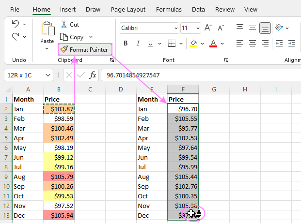
- When done, press Esc to stop using the paintbrush.
- Select any cell in your new dataset, open the Rules Manager and check the copied rule(s).
Note. If the copied conditional formatting uses a formula, you may need to adjust cell references in the formula after copying the rule.
How to delete conditional formatting rules
I've saved the easiest part for last :) To delete a rule, you can either:
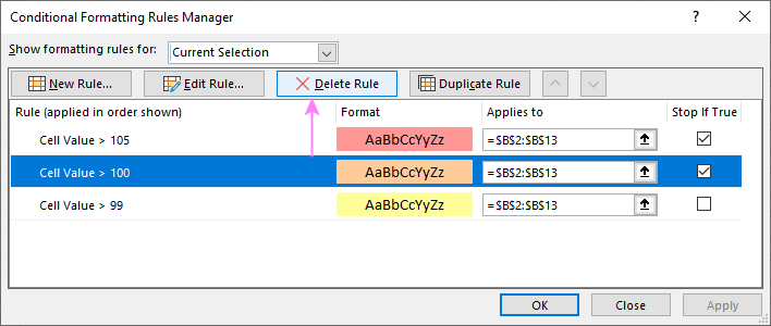
- Open the Conditional Formatting Rules Manager, select the rule and click the Delete Rule button.
- Select the range of cells, click Conditional Formatting > Clear Rules and choose the option that fits your needs.

This is how you do conditional formatting in Excel. Hopefully, these very simple rules we created were helpful to get a grasp of the basics. Below, you can find a few more tutorials that can help you understand the inner mechanics and expand conditional formatting in your spreadsheets far beyond its traditional uses.
Practice workbook for download
Excel conditional formatting - examples (.xlsx file)
 by
by
310 comments
How can we add value of two cell but show in one cell
For exmpl
A1 cell value is 10
B1 cell value is 20 total 30(a1+b1)
But these values calculated in b1 cell not another cell. Plz reply
Hi,
I'm sorry, but it's impossible to show the number AND the sum of numbers in a cell at the same time.
Sir/Mam
I have 2 question.
1:- When I will enter date in shhet2 A2 column then the out put will show in sheet2 B2 column. My B2 column formula is =If(isblank(A2),"Please enter Date",if(isnumber(A2),vlookup(A2,Sheet1!A:C,2,0),"Invalid Date")).
So I want, when will show "PLEASE ENTER DATE" in B2 then the font colour will be GREEN. When "INVALID DATE " will show then the font colour will be RED.And the result of vlookup font colour will show YELLOW.
2:- The second question is- I put the formula in B6 =if(A6="Sun","Ashok,Deepak",if(A6="Mon","Rajesh,Ramesh",if(A6="Tue","Prakash,Dillip",""))).
So I want when the name will show then the font colour will be blue.
so please tell me how to solve it by conditional formating.
Hello Experts..
I have a table in which I already inserted formula & conditional formatting to get the result.
Example:- In column O3 I have mentioned Expiry Dates & in column P3 I have mentioned =O3-TODAY() & inserted conditional formatting to know remaining days to get expired with Less than value using colour format. (Like, colour to be change as yellow if days remain less than 60 & Red if days remain less than 30) it is working.
But What I want is if the expiry date has not mention in column O3 then Column P3 should be blank without anything.
Hello Friends!
I writing the figure 624 in a cell G6 and in cell H6 I writing =G6*1% in this case I got the correct answer, but I intend to get formula for multi figures in h6 like this =g6*1% with the new answer *10% and further with new answer *12% in just a single cell as H6. what I can do for the same. Guide me someone please.
M. Munir
KINDLY IGNORE A1 =.
THANKS
R/MAM,
GOOD NOON,
PL NOTE THAT A1 CELL HAS A VALUE "X", I WANT TO HIGH LIGHT CELL B1 WHEN IT'S VALUE LESS THAN 10% OF CELL A1.
IN FORM OF MATHS
CELL B1 SHOULD BE HIGHLIGHT WHEN
A1 = < A1-(A1*0.1)
HOW CAN I DONE BY CONDITIONING FORMATTING FACILITY?
REGARDS,
MONIK
How do I get excel to calculate the difference in dates in days?
Thank you
Kenny
Hi Kenny,
You can use the DATEDIF function with the "d" unit, as shown in this example:
How to calculate difference between 2 dates in days
I have a training spreadsheet with expiry dates. I want to use traffic lights to turn the cells red, amber or green as they approach the date of expiry compared to todays date, in months. eg due in 12 months or more green, due in 6 months or more amber and less than 6 months red. Is there an easy way to do this in Excel 2010 please. I have formatted the date as eg Jan 2017, Mar 2019 to make it easier. Thanks
Hello,
I've been trying to make this work. I want that every time I have a negative number in column L, the whole row where the number is change the font to red. I can make it work for just one row but when I try to implemented in the worksheet is when I got stuck. In the conditional formatting option I select the "Use a formula..." option. I type =$L:$L<0, But it doesn't work. when I just select a specific cell (i.e. =$L$145), it works but that's not what I am looking for. On the other part I just type the rows I want to be affected by this (=$A:$R,$T:$AD).
Any help regarding this matter, I really appreciate it.
Thank you!
Hi Guys, Can someone help me please.
i need help with an example below.
i want in column x. 13/06/05 , 14/08/16, 25/07/17
in column y i want it to turn red if nothing is filled in a week after the dates in column x.
Can someone please help
im building 5 town houses, i owe the bank 2.5 million
when i have sell for 5 townhouses lets say 600- 700 thousand each
in excel i got
2.5m in cell B3
every time i sell a house i enter the price and it deducts from B3
lets say i have 300 thousand left to pay off showing in B3
i enter 400 thousand i want the B3 to be zero and what is leftover goes to a different cell
hope this makes sense
Hi
i have names lised in a column 1-15.
What i am trying to do is is, that if one of those same names appears in another cell in the same column, that the original name in the column 1-15 disappears and turns a different colour?
Is this possible through conditionl formatting?
Ray
Hello
I need help.
I want to see only one cell in which conditional formatting applied on the basis of value entered in the cell.That means if i enter 10% then 10% of the cell will coloured, if i enter 50% then 50% will be colored,if i will enter 100% then full cell will be coloured.(This is for only one cell).
Thanks in advance.
I'm trying to make a timecard that calculates both regular and overtime hours. I want to make it where when I reach a total of 40 hours in regular time it stops entering data in the cells in the regular time column and any time over 40 hours will then start showing up in the cells in the overtime column.
I apologies if this doesn't make sense
Hello!,
I am designing a hitmap using conditional formatting and I would like not to show the value in the cell. I have tried modifing the format of the cell by writting the comand ;;;; in the costum blog of the cell format... but does not work... any idea on how to "Hide" the cell value?
Thanks
How to Get? - If amongst 4 cells if I put 1 in any of the cells, rest of the three cell should be showing 0. How to do that?
Which formula to use?
hi
i have series of rows employee wise , with character p entered for present on applicable dates in a month , i want to highlight the column where p consecutively appears in a row 10th time
Hi,
i want to learn how to make alert(thru highlight) when the stocks was below safe level. i was able to find out how for 1 row but my problem was how to do it if i'm monitoring 1 thousand items wherein i don't have to do it 1 by 1. 2nd, is it possible to highlight the entire row?
example
item on hand safety stock
a1 10 15
a2 11 14
....
a1000 12 10
Hi, Edilberto,
if C column indicates safety stock and it should not (ideally) exceed the number of items on hand (column B) then the formula for conditional formatting rule is:
=$C1<$B1
and it applies to =$A:$C.
It will also highlight the raw if C is empty.
If you want something other than that, please, specify.
Also, here is a great tutorial on how to highlight an entire raw.
Hi,
Can someone please help me. I need to do conditional formatting on values that are on different worksheets.Cell O5 in worksheet A if it's found in Cell I in worksheet B to be highlighted as whatever colour.
Many thanks
hi
I need to be able to register in two cells the highest and lowest negative and positive results from a changing portfolio total in order not to have to manually monitor and record these myself. I am a complete novice when it comes to formatting cells so a simple abc approach would be very much appreciated.
Many thanks
Hi, David,
let's say that your totals are in the 7th row (A7:G7). And you have two other cells where you want to see the highest and lowest results. So, for the lowest one you put the next formula in the cell:
=MIN(A7:G7)
(where A7:G7 is your range of the results)
For the highest one, enter another formula in another cell:
=MAX(A7:G7)
Every time the results change, these formulas will adjust the highest and the lowest numbers.
If you need to find the lowest AND the highest for negative results, the lowest AND highest for positive ones, let us know what Excel version you're currently using.
Natalla
Many thanks for your advice, much appreciated.
I may not have explained the problem correctly. I have one cell with an ever-changing total, both post and neg, which I record in two other cells, one recording the highest positive and the other the highest negative. I would like to be able to record these automatically so need the formula for each cell to do that.
I am using Excell for Mac 2011 version 14.7.3
Apologies for any misunderstanding and thanks once again
Hi team
i have a doubt regarding the average of values, for suppose if we have two trials TS1 and TS2, in which i have got TS1 is 0.08% and TS2 is 0.03%, the average we required is from the values which are >0.05% it means the final value from above is 0.08%. for this i have kept a command that =IF(AVERAGE(D14,F14)<0.05,"<0.05",AVERAGE(D14,F14)). for suppose the values for TS1 and TS2 both are <0.05% it means if TS1 is 0.03 and TS2 is 0.04 then the Average value to be displayed is <0.05. but iam not able to get it, plz anyone can help me out.....
Hy Svetlana
Today I Read Your excel formula where i am very pleasant because you solve many people problem i need some help
example
i create timing report
( Like )
Real In Time: Employ In Time (Remarks)
9:00 9:25 late
9:00 9:28 late
9:00 9:18 OK
9:00 9:22 late
i want formula which show automatically status if employ 20 mint late come
Good day. Please assist me as i have to insert an IF formula for an evaluation tool. I have an overall average calculated for the tool however i require an IF formula that states if a certain criteria = 0 then the overall evaluation average should =0.
Hi Svetlana
I used your instructions for conditional formatting, which worked wonderfully, thank you! However, I'm now stumped as to how to copy these colours over, I will try to explain:
Used the formatting to fill colour in cells of varying "greater than" amounts relating to an average value which is based on a figure entered each week. So the names of people are down column A and each column after has their weekly score. Column AA has the average, which is coloured accordingly. I'd like to have the cell containing the name of each person to automatically fill with the same colour as the one containing their average score.
I am a complete novice at this, hope you can help :)
I have a column with data in it with 3 rules set up. The rules are if the value is less than 80, highlight the cell in red, if the value is between 80 and 89, highlight in yellow and if the value is between 90 and 100, highlight the cell in green. Everything works as it should. I would like to know if it is possible to create another conditional format rule for all cells to the right of my column with values in it that will highlight the cells for each line of data to change color based on the data column?
I only want to input values in the one column all the way to the left. The rest of the columns to the right only change color based on that column of cells.
please send your mail id. i want to send a spread sheet to you. That's my worksheet for deviation statement for govt sector. i need your hepl to fixing the formula in this worksheet. thanking
Is it possible to get copies of the workbooks you use in your conditional formatting articles so I can practice?
I want use to Conditional formatting
If A Column is "Sunday",
Then B Column Fill Red color. Is this possible
Thank you Irina.
I want to implement alternating rows conditional formatting only if a field in Column A (A5:A500). Please help how I can achieve that? The formatting that I want to include is adding a border and filling the cell with a colour. Cheers.
Hi
I have a column that I want to apply data bar conditional formatting to, however when I apply the formatting it doesn't appear. The data is calculated from other cells and contains formulas. Kindly assist
Regards
Hi,
I am working on a spreadsheet which is to show delays in projects. I am using conditional formatting formulas to change the colour of the cell directly beneath the planned week number.
Is there a way to copy this format so that the reference cells are automatically updated as they would be if a copying a normal formula?
Thanks
Steve
Hello, I have a large spreadsheet with columns of data (example, K 39,041.00, L 34,584,.25, M 26, N 39,470.04)and would like to highlight cells in both column K & N if column N is greater than column K. I would like to do the same thing (different color) if column L is equal to column K. Can I accomplish this through Conditional Formatting?
Thanks in advance,
Jeff
Hi there,
I have list of codes in tab 1 (approx 100). I want to format the colum A in tab 2 that if I type the code other than mentioned in tab 1 than it should highlight.
Will conditional format will work on this occasion?
Regards,,
Hi Sandeep,
Sure, you can use the following formula for your Conditional Formatting rule to highlight values that differ:
=AND($A2<>"",COUNTIF($A2, Sheet1!$A$2:$A$150)=0)
You can also compare the date with Duplicate Remover add-in to find unique values in your second sheet.
Hi,
I need to give me a reminder or change color of the vehicle ID colomn as soon as it reaches the oil change mileage. I have to develop a worksheet for oil change of fleet of vehicles. The oil change is based on current mileage to next mileage which is (Current Mileage + 7000). Would you help me out with this one.
THanks
Hello Afaq,
Could you please describe the structure of your table in more detail? Do you have columns with the IDs, current mileage, and mileage of the last time oil was changed? We'll do our best to assist you.
Hello,
I have a worksheet of inventory items. The first column is the stock number the second is the name of the items. The third one is how many we have received. The other columns are items that went to a project, we have approximately 13 projects and a formula for the last two columns which have what has been issued and what is available. The problem arises when my boss wants to lock the third column C which has the number of items purchased that has been sent to us. I have tried using the page protection function, but this locks the whole page not just the items in column C. I need the rest of the page to function while locking a single column. Is that possible and if so how do I do it?
Hello Ray,
You can lock any range in your sheet, this feature is quite flexible in Excel. Please see detailed steps in this support article.
Hello experts!
I want a conditional formatting in following context:
1. I have 6 columns and more than 30 rows.
2. Column A contains dates in English & column B contains dates in local language.
3. Column C contains days as "Sun", "Mon"......
Here, I need a conditional formatting of cells from Column A through Column F if column C contains "Sat". This condition should apply even in blank cells where I need "cell fill color".
Problem: I can fill color in the cell containing "Sat" but I need the same in entire row from column A up to F.
Can somebody help me out?
Thank you
Hello Bhagirath,
You need to create a rule with a formula, here are the steps:
- Select the range with your data, e.g. A2:F100
- Click on "New Rule" under Conditional Formatting and select the last option: "Use a formula to determine which cells to format"
- Pick format for the rows and enter the following formula:
=$C2="Sat"
This blog post describes how to format entire rows based on values in certain cells:
https://www.ablebits.com/office-addins-blog/excel-conditional-formatting-formulas/
I have some numbers,with seperate cells. if i select one digit, automatically
that shows how many same digits in that page. with Bold & Colored. ?
please
I have created a sales sheet with description,price,quantity,and total with 5 different product that I sell. Now I want to create another, where when I sell any item the system will automatically calculate the total of so I can save. Thus POS but I will not print a receipt
I want a cell to turn red base on a response in a combo box. The formatting works when it is in relation to any other cell or even a drop down list, but it seems as if it is not recognizing the combo box.
884,00
125,00
4,15
4,15
1,00
9,46
1,56
1,13
25,00
3,75
1,00
1,00
1,13
5,00
6,88
2,36
1,06
2,55
2,48
6,16
7,50
1,88
102,50
168,75
0,37
0,11
0,92
2,31
7,50
0,46
1,13
3,75
6,50
3,40
1,31
26,25
1,31
1,75
25,00
3,90
hi above value which is i want to sum but the value occurs always zero,please get me solution
Put these values column A
use below formula and drag down
=VALUE(SUBSTITUTE(A1,",",""))
then Use Sum function
I have at the top today date
I have around 30 rows where i have typed different dates. I want to highlight if the row date is less than today date with red font. Kindly help me how to do this.
Regards,
Guddappa nadiger
IN EXCEL ONE COLUMN MATERIAL SEND DATE,NEAREST COLUMN DATE TODAY ,NEXT COLUMN COUNT DATE FROM 1 TO 2 COLUMN,NEXT COLUMN DAYS>180 MEANS INDICATES RED
DAYS<180 MEANS INDICATES GREEN
NEXT COLUMN ACTUAL DATE OF RECEIVING,NEXT COLUMN STATUS OPEN/CLOSED(IF MANUAL ENTER ACTUAL DATE OF RECEIVING MEANS)THAT AUTOMATICALLY COMES CLOSE THEN DATE FORMULA WILL NOT UPDATE FOR THAT PARICULAR ROW
how to running value control via condition formatting a1-10then b1 100,c1 200 but my total is 300 i want a1 greater then b1 then highlight b1
Hi I excel sheet if there are 10 employees I'd in column and in other excel sheet i want the employee I'd twice. Is there any formula for same
Hi
why my file cannot save the custom conditional formatting?
How to I highlight a column cell if the minute value is within 15 minutes of another column cell?
Example:
C4 is 9/30/16 12:11
F4 is 9/30/16 12:23
C4 is only 11 minutes before F4 and needs to be highlighted.
Thanks
Hi,
Could you tell me how to use conditional formatting to turn one cell yellow 5 minutes before to five minutes after the time "now()" listed in second or different cell?
which formula we used in condition formation to coloring the amount is greater than 30 and less than 61
Hello,
You need to use the following formula:
=AND($A2>30,$A2<61)
How can I get the total in two cell's to reduce when I add an amount in another cell?
For example cell H7 is at 100 and cells M7 and N7 are at 20. When I make cell H7 105 how can I automatically get cells M7 and N7 to reduce to 15? The cells are in hours and minutes.