In this tutorial, you will learn a few different ways of copying formulas in Excel - how to copy formula down a column, to all of the selected cells, copy a formula exactly without changing cell references or formatting, and more.
Copying formulas in Excel is one of the easiest tasks that is usually done in a mouse click. I say "usually" because there can be very specific cases that require special tricks, like copying a range of formulas without changing cell references or entering the same formula in multiple non-adjacent cells.
Luckily, Microsoft Excel offers many ways to do the same task, and it is true for copying formulas. In this tutorial, we are going to discuss different ways to copy formulas in Excel so that you could choose the one best suited for your task.
How to copy formula down a column
Microsoft Excel provide a really quick way to copy a formula down a column. You just do the following:
- Enter a formula in the top cell.
- Select the cell with the formula, and hover the mouse cursor over a small square at the lower right-hand corner of the cell, which is called the Fill handle. As you do this, the cursor will change to a thick black cross.
- Hold and drag the fill handle down the column over the cells where you want to copy the formula.
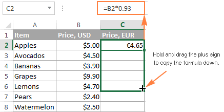
In a similar manner, you can drag formula into adjacent cells to the right, to the left or upwards.
If the formula includes relative cell references (without the $ sign), they will automatically change based on a relative position of rows and columns. So, after copying the formula, verify that the cell references have got adjusted properly and produce the result that you want. If necessary, switch between absolute, relative and mixed references by using the F4 key.
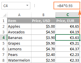
In the above example, to make sure the formula was copied correctly, let's select some cell in column C, say C4, and view the cell reference in the formula bar. As you can see in the screenshot below, the formula is all right - relative to row 4, exactly as it should be:
How to copy a formula down without copying formatting
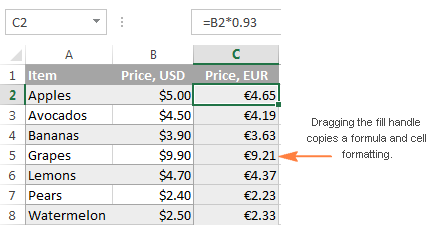
Copying a formula down by dragging the fill handle not only copies the formula, but also the source cell formatting such as font or background color, currency symbols, the number of displayed decimal places, etc. In most cases, this works just fine, but sometimes it can mess up the existing formats in cells where the formula is being copied to. A common example is overwriting alternate row shading like in the following screenshot.
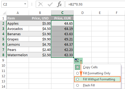
For prevent overwriting the existing cell formatting, drag the fill handle as demonstrated above, release it, click the Auto Fill Options drop-down menu, and select Fill Without Formatting.
Copy formula to the entire column
As you've just seen, the fill handle makes copying formulas in Excel really easy. But what if you need to copy a formula down a ten-hundred-line sheet? Dragging the formula over hundreds of rows does not look like a good idea. Luckily, Microsoft Excel provides a couple of quick solutions for this case as well.
Double-click the plus sign to fill the whole column
To apply the formula to the entire column, double-click the plus sign instead of dragging it. For those who have skipped the first section of this tutorial, the detailed steps follow below.
To copy an Excel formula to the whole column, do the following:
- Input your formula in the top cell.
- Position the cursor to the lower right corner of the cell with the formula, wait until it turns into the plus sign, and then double-click the plus.
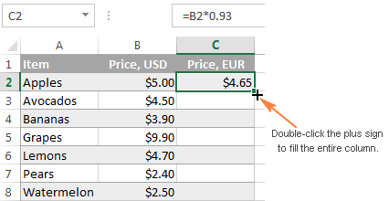
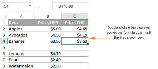
Note. Double-clicking the plus sign copies the formula down as far as there is some data in the adjacent column(s). As soon as an empty row occurs, the auto fill stops. So, if your worksheet contains any gaps, you will have to repeat the above process to copy the formula below an empty row or drag the fill handle as explained in the previous examples:
Create an Excel table to copy a formula to all cells in a column automatically
Among other great features of Excel tables such as predefined styles, sorting, filtering and banded rows, automatically calculated columns is what makes an Excel table a truly wonderful tool for analyzing groups of related data.
By entering a formula into one cell in a table column (just any cell, not necessarily the top one), you create a calculated column and have your formula instantly copied to all other cells in that column. Unlike the fill handle, Excel tables have no problem with copying the formula across the entire column even if the table has one or more empty rows:
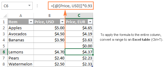
To convert a range of cells to an Excel table, simply select all the cells and press Ctrl + T. If you prefer a visual way, select the range, go to the Insert tab > Tables group on the Excel ribbon, and click the Table button.
Tip. If you don't really want an Excel table in your worksheet, to can create it temporary, to make the work with formulas easier, and then you can convert the table back to a usual range in a second. Just right-click the table and choose Table > Convert to Range in the context menu.
Copy a formula to non-adjacent cells / ranges
It goes without saying that the fill handle is the fastest way to copy formula in Excel. But what if you want to copy your Excel formula in non-contiguous cells or beyond the end of the source data? Just use the old good copy & paste way:
- Click the cell with the formula to select it.
- Press Ctrl + C to copy the formula.
- Select a cell or a range of cells where you want to paste the formula (to select non-adjacent ranges, press and hold the Ctrl key).
- Press Ctrl + V to paste the formula.
- Press Enter to complete the pasted formulas.
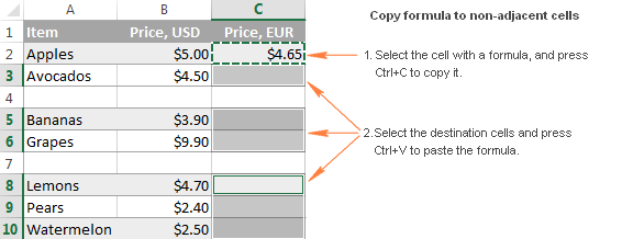
Note. The copy/paste shortcuts copy the formula and formatting. To copy the formula without formatting, choose an appropriate Paste option on the ribbon or in the right-click menu, as demonstrated in Copying an Excel formula without formatting.
Enter a formula into multiple cells with a single key stroke (Ctrl + Enter)
In situations when you need to input the same formula in more than one cell on a worksheet, adjacent or non-adjacent ones, this method can be a time-saver.
- Select all the cells where you want to enter the formula. To select non-contiguous cells, press and hold the Ctrl key.
- Press F2 to enter the edit mode.
- Input your formula in one cell, and press Ctrl + Enter instead of Enter. That's it! The formula will get copied to all of the selected cells, and Excel will adjust relative cell references accordingly.
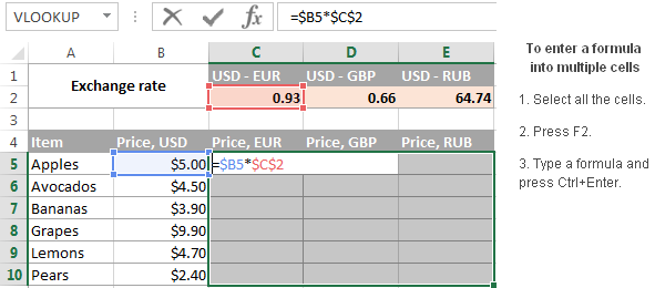
Tip. You can use this method to enter any data, not just formulas, in multiple cells at a time. A few other techniques are described in the following tutorial: How to enter the same data into all selected cells at a time.
How to copy an Excel formula but not formatting
As you already know, when copying a formula down a column in Excel, you can use the Fill Without Formatting option that lets you copy the formula but keep the existing formatting of the destination cells. Excel's Copy & Paste feature offers even more flexibility with regard to paste options.
- Select the sell containing the formula.
- Copy that cell by pressing Ctrl + C. Alternatively, right click the cell and select Copy from the context menu, or click the Copy button on the Home tab > Clipboard.
- Select all the cells to which you want to copy the formula.
- Right-click the selected cells and choose Formulas under Paste Options:
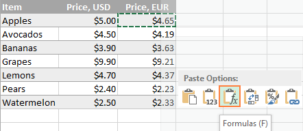
For more paste options, click the arrow below the Paste button on the ribbon. For example, you can select Formulas & Number Formatting to paste only the formula and the number formatting such as percent format, currency format, and the like:
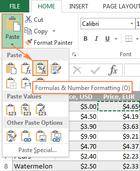
Tip. If you are not sure which paste option works best for you, hover the mouse over different icons to see a preview of this or that paste option.
Copy formula in Excel without changing references
Excel formulas rarely occur in a spreadsheet in solitude. In most cases, you enter a formula in one cell, and then copy it to other cells in the same column or row, to perform the same calculation on a group of data. And if your formula contains relative cell references (without $), Excel automatically adjusts them so that each formula operates on data on its own row or column. Most of the time, this is exactly what you want. For example, if you have the formula =A1*2 in cell B1, and you copy this formula to cell B3, the formula will change to =A3*2.
But what if you want Excel to copy the formula exactly, without changing the cell references along the way? Depending on your particular task, choose one of the following solutions.
Copy or move a single formula without changing cell references
If you need to copy or move just one formula, making an exact copy is easy.
- Select the cell with the formula you want to copy.
- Select the formula in the formula bar using the mouse, and press Ctrl + C to copy it. If you want to move the formula, press Ctrl + X to cut it.
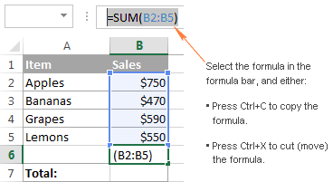
- Press the Esc key to exit the formula bar.
- Select the destination cell and press Ctl + V to paste the formula there.
Alternatively, you can enter the editing mode and copy the formula in the cell as text:
- Select a cell with the formula.
- Press F2 (or double-click the cell) to enter the editing mode.
- Select the formula in the cell using the mouse, and press Ctrl + C to copy it.
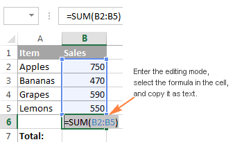
- Select the destination cell, and press Ctl+V. This will paste the formula exactly, without changing the cell references, because the formula was copied as text.
Tip. To quickly copy a formula from the above cell with no reference changed, select the cell where you want to paste the formula and press Ctrl + '.
Copy a range of formulas without changing cell references
To move or copy a range of Excel formulas so that no cell references are changed, use one of the following methods.
Method 1. Use absolute or mixed cell references
If you need to make an exact copy of formulas with relative cell references (like A1), the best way would be changing them to absolute references ($A$1) to fix the reference to a given cell, so that it remains static no matter where the formula moves. In other cases, you may need to use mixed cell references ($A1 or A$1) to lock either a column or row. Doesn't make much sense so far? Okay, let's consider the following example.
Supposing, you have a table that calculates the fruit prices in EUR based on the USD price in column B and the exchange rate in cell C2:
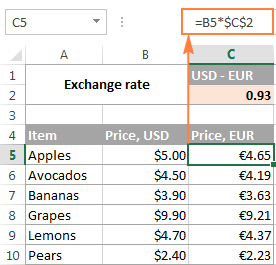
As you can see in the screenshot above, the formula includes an absolute cell reference ($C$2) to fix the exchange rate to cell C2, and a relative cell reference to cell B5 because you want this reference to adjust for each row. And this approach works well as long as the formulas remain in column C.
But let's see what happens if you need, say, to move the EUR prices from column C to column F. If you copy the formulas in a usual way by copying/pasting the cells, the formula from cell C5 (=B5*$C$2) will change to =D5*$C$2 when pasted in cell F5, making your calculations all wrong!
To fix this, just change a relative reference (B5) to a mixed reference $B5 (absolute column and relative row). By putting the dollar sign ($) in front of the column letter you anchor the reference to column B, no matter where the formula moves.
And now, if you copy or move the formulas from column D to column F, or any other column, the column reference won't change because you locked it by the dollar sign ($B5).
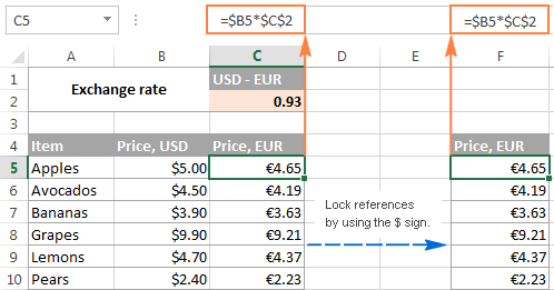
The concept of Excel cell references may be difficult to grasp from the outset, but trust me it's worth your time and effort because it will save you much more time in the long run. For example, see how you can calculate the entire table with a single formula by using mixed cell references.
However, if you already have a ton of formulas with relative cell references in your Excel sheet, and you need to quickly make an exact copy of those formulas but you don't feel like you can get the references right, one of the following methods could be a solution.
Method 2. Copy Excel formulas without changing references via Notepad
- Enter the formula view mode by pressing the Ctrl + ` shortcut, or by using any other method described in How to show formulas in Excel.
- Select all the cells with the formulas you want to copy or move.
- Press Ctrl + C to copy the formulas, or Ctrl + X to cut them. Use the latter shortcut if you want to move formulas to a new location.
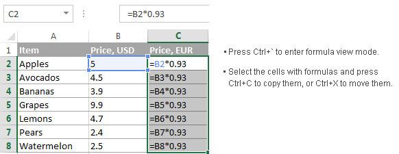
- Open Notepad or any other text editor and press Ctrl + V to paste the formulas there. Then press Ctrl + A to select all the formulas, and Ctrl + C to copy them as text.
- In your Excel worksheet, select the upper-left cell where you want to paste the formulas, and press Ctrl + V.
Notes:
- You can paste the formulas only in the same worksheet where your original formulas are located, unless the references include the sheet name, otherwise the formulas will be broken.
- The worksheet should be in formula view mode. To verify this, go to the Formulas tab > Formula Auditing group, and check if the Show Formulas button is toggled on.
- After pasting the formulas, press Ctrl + ` to toggle off the formula view mode.
Method 3. Copy formulas exactly by using Excel's Find and Replace
To copy a range of Excel formulas without changing their cell references, you can use the Excel Find and Replace feature in the following way.
- Select the cells with the formulas that you want to copy.
- On the Home tab, go to the Editing group, and click Find & Select > Replace… Or, simply press Ctrl + H, which is the shortcut for launching the Find & Replace dialog in Excel.
- In the Find & Replace dialog window, type the equal sign (=) in the Find what box. In the Replace with box, input some symbol or a string of characters that is not used in any of your formulas, like ', # or \.
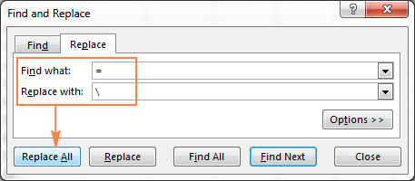 The purpose of this step is to turn formulas into text strings, which will prevent Excel from changing the cell references during the copy process.
Note. Do not use an asterisk (*) or question mark (?) for replacement, since these are wildcard characters in Excel and using them would make later steps more difficult.
- Click the Replace All button and close the Find and Replace dialog. All the formulas in the selected range will turn into text strings:

- Now, you can select any cells, press Ctrl + C to copy them, select the top cell in the current worksheet where you want to paste the formulas, and press Ctrl + V. Since Excel does not interpret the formulas without the equal sign as formulas, they will be copied exactly, without changing references.
- Use Find & Replace again to reverse the change. Select both regions, with the original formulas and copied ones (to select non-adjacent regions, press and hold Ctrl). Press Ctrl + H to open the Find & Replace dialog. This time, enter the back slash (\) (or any other character you used for the first replacement) in the Find what box, and = in the Replace with box, and click the Replace All button. Done!
Shortcuts to copy Excel formula to other cells
1. Copy a formula down
Ctrl + D - Copy a formula from the cell above and adjusts the cell references.
For example, if you have a formula in cell A1 and you want to copy it to cell A2, select A2 and press Ctrl + D.

2. Copy a formula to the right
Ctrl + R - Copy a formula from the cell to the left and adjusts the cell references.
For example, if you have a formula in cell A2 and you want to copy it to cell B2, select B2 and press Ctrl + R.

Tip. Both of the above shortcuts can be used to copy formulas to multiple cells too. The trick is to select both the source cell and target cells before pressing the shortcut. For example, if you want to copy the formula from A1 to the next 9 rows, select cells A1:A10 and press Ctrl + D.
3. Copy a formula down exactly
Ctrl + ' - Copies a formula from the cell above to the currently selected cell exactly and leaves the cell in edit mode.
This is a quick way to make an exact copy of a formula without changing cell references. For example, to copy a formula from cell A1 to A2 so that no references are changed, select A2 and press Ctrl + '.
Note. Don't confuse the shortcut Ctrl + ' (Ctrl + single quote) that exactly copies a formula from the cell above with Ctrl + ` (Ctrl + grave accent key) that activates show formulas mode in Excel.

Well, this is all I have to say about copying formulas in Excel. If you know some other methods to quickly move or copy formula in Excel sheets, please do share. I thank you for reading and hope to see you on our blog next week!
 by
by
198 comments
I am working on a scoresheet for athletic events. I have multiple weight classes. I have 7 events and overall score and rank in each weight class. I'm using "=IF(G18>0,(IFERROR(RANK(G18,G$18:G$37,IF(G$16="Low",0,1)),0)),)" to figure the points awarded for each event. How do I copy the entire weight class worth of formula to a new weight classes? Every time I try, it will change the G18 but not the G$18:G$37, which should be G39,G$39:G$58 after copying.
Hello
I would appreciate your help.
For some reason I cannot paste a formula ONLY into the same cell in a different worksheet (same file) and have the cell references automatically adjust. It only pastes the exact same formula. These are simple formulas:
=SUM(M9:M14). So instead of this formula adjusting to the rows say M9:M21 it stays at M9:M14. I don't remember this being that way - is there something I did that made this happen? The cells adjust if I do that in the same worksheet but NOT between worksheets.
Thank You, James
Hi
I have a question what if you are dragging down and the formula is not showing the updated result, how do I return to the mode where dragging down a formula within the cell allows me to copy but the results will be updated as well
thanks
Under the section "How to copy formula without changing references" your Method 2 is brilliant and totally new to me. It saved me a couple of hours of tedious and error-prone labor. I would gladly pay $75 for the help you have given me. Is there a way?
Jim J.
> Hi! Great article! The Best in The Web! Congratulations & Respect! :-)
>> One 'Add-in':
>>> Ref. above sections: "Copy a range of formulas without changing cell references" & "Create an Excel table...":
In order to copy whole column of formulas intact, in other words to 'duplicate' them:
Create Table / Make formula, in a cell of a column adjacent to the Table, referring to Table's several columns - then: Table automatically expands to this cell and column and copies formula to this whole new column / select this new column of formulas / copy it to the next adjacent column outside the Table / Voila!: the formulas in the newest column are copied exactly the same as they are in the previous one - with no change of references!
> Hope it will help! BstRgds.AR:-)
Thanks useful.
I'm trying to create a formula for a basic point of sale type stock control sheet. I'm using the IF function to pull prices from the purchases sheet into the recipes sheet, but I'm finding that if I need to add or remove stock items to the purchases sheet, deleting rows knocks out my formula - probably because I am using absolute references in my IF formula: =IF(Purchases!$A$5="Avo";Purchases!$W$5;0). I've been looking up the Excel INDIRECT formula, but am struggling to make head or tail of the tutorials I've read online - can anyone tell me how to create a formula that will keep the cell references as they are without regardless of whether or not I am deleting rows? Any help would be appreciated!
this kind of formula is the best!!!!
Thank you for the helpful tips...found exactly what I was looking for!
Hi, I am trying to copy a formula from say cell A1 that has references from another Data source tab (say C1). I want to copy cell A1 and paste it in say cell A9 in the same sheet but want the cell reference in the formula to change by one row in the Data Source tab (from C1 to C2). How do I do this?
Thank you so much! was reading all these different forums and every answer seemed excessively complex, 10 seconds into this page and you got it in one :)
i would like to drug down a formula. it gives varring values correspondning to the intededed cells for a certain range downwards. but after that range the calculated values are the same regardless of variations in the in the data being calculated. please help
I have got a Cash Flow Analysis Workbook that reorts on Daily, Weekly and Monthly values. When I wish to extend the spreadsheet, the Daily values are a simple copy / paste. However, on the Weekly analysis Worksheet, I need to jump 7 columns each time for the totals (i.e. Copying A1 to the next column gives me B1 when I actually need H1) I have the same issue with the monthly analysis Worksheet when I need to go from A1 to AD1 in the next column. Is there a simple way to copy with this jump on references or is it a case of manually amending the references each time|?
I have an Excel spreadsheet which I made last year for a luncheon with about 300 people. I linked a page to it which creates name badges, using some of the information from the first list. This is an annual function and this year we would like to change the font on the name badges. I have created formulas so that if I change a line on the first badge, all of the badges will change as well. However, if I change the font on the first badge, no other badges will change fonts. Only the wording changes. How I get the font on all of the badges to change at one time to whatever is in that first badge? We will be using this spreadsheet for many years to come, but would to occasionally change the font, and I know there must be an easier way other than copy and paste! Thank you in advance for your help.
HEY GUYS. I THOUGHT THIS MIGHT BE HELPFUL I DID THIS IN ALL CAPS ON PURPOSE...
FOR ALL THOSE WHO WANT TO COPY A RANGE OF CELLS WHILE KEEPING THE REFERENCES(THIS IS IMPORTANT CAUSE IT CAN SAVE A LOT OF TIME WHILE EDITING)
I'M NOT SURE IF IT WAS MENTIONED IN THE TUTORIAL ABOVE BUT WHILE READING I GOT IMPATIENT AND TRIED THIS AND IT WORKED... WELL HERE GOES.
FIRST COPY THE ENTIRE WORKBOOK THAT THE CELLS ARE, IN FOR THOSE WHO DON'T KNOW HOW TO.. GOOGLE IT IT'S EASY.. THEN ONCE IN THE COPIED WORKBOOK "CUT" THE CELLS YOU WANT AND PASTE THEM IN THE ORIGINAL BOOK WHERE DESIGNATED... EASY PEASY
Dude, you just save my work life!!! Thankssss
Hello. I am trying to help a friend with an Excel sheet. At this time his sheet looks like this: The numbers under the month represent the number of people with these reasons. All of a sudden, the boss wants it in a different format, and i can't get it where it needs to be for him.
Right now it is like this:
County Reasons Jan Feb March April May
Adams Don't want 4 0 5 2 3
Benton Don't have 0 4 7 8 2
Benton Don't like 1 1 1 1 1
Boss wants it like this -
County Reasons Month Clients
Adams Don't want Jan 4
Adams Don't want Feb 0
Adams Don't want Mar 5
Adams Don't want April 2
We have 39 counties and 10 possible reasons and 12 months. When I used the INDEX function, transpose or anything else, I just could not make it work. I don't want to have to write this all manually. It's impossible. Happy to work by phone if easier. Just let me know.
how can i achieve this kind drag increment
'=IF(B7>D7,A7,IF(D7>B7,E7))
'=IF(B9>D9,A9,IF(D9>B9,E9))
,=IF(B11>D11,A11,IF(D11>B11,E11))
,=IF(B13>D13,A13,IF(D13>B13,E13))
and so on...
Well done dear,
Excellent Job. thanks so much for supporting the learners.
1. Cut the Range of formulas.
2. Paste itin the new location.
3. Copy the contents, from the new location, that you just pasted.
4. "Undo" the Cut-Paste operation (this will put the original content back to the original range).
5. Paste the contents from the Clipboard(!) to the new desired location (Like 2 above).
(The formulas will have the original references).
IF it looks like a lot of work – take a look at the keyboard shortcuts:
1. Ctrl-X
2. Ctrl-V
3. Ctrl-C
4. Ctrl-Z
5. Ctrl-V
--------------------------
Michael (Micky) Avidan
“Microsoft® Answers" - Wiki author & Forums Moderator
“Microsoft®” MVP – Excel (2009-2017)
ISRAEL
"W.O.228WO No-228 (Location.2.109/ Town Center) 21" in this value i want copy only 2.109 this is the word no 28-31 please tell me formula
Pls help, i must copy a lot of cell info from 1file to another, downwards. But if i copy a range downwards and past it does not copy it in seq
Ect
+'[file name]'!$j$3
And i select a range it only copy to the next range on new file +'[file name]'!$j$3 on all cell but i want it to be +'[file name]'!$j$4. +'[file name]'!$j$5. Pls help. Regards
I would like to copy a changing daily value as it moves down a column in my main worksheet to a single cell in another tab. The cell location in this other tab always remains in this one location.
Thank you for any feedback.
Craig
I would like to copy a changing value as it moves down a column in my main worksheet, to a single cell in a separate tab. It will not change cells in the separate tab but always copy to this single cell while it still changes daily in the main worksheet.
I have a form on sheet 1. All the the raw data's i have are all on sheet 2 (all reference). When i enter a number on the form (Sheet 1) the information automatically goes to Sheet 3. What i'm thinking is how can i not make the result on Sheet 3 not disappear when i clear out the form on Sheet 1? and when i fill out the form on Sheet 1 again, how will i make the result be put on the next row on Sheet 3? Please help me...:-(
These explanations are worthless. (1.) Nowhere does it tel us how to copy a back of cells and paste them somewhere without changing cell references, if even if that is possible or not in EXCEL. It is such a common need that it is ridiculous no to address it.
(2.) The method of explain things is at sea. What die sit mean to:
Ctrl + R - Copy a formula from the cell to the left and adjusts the cell references.
For example, if you have a formula in cell A2 and you want to copy it to cell B2, select B2 and press Ctrl + R.
What else if happening when you type Ctrl + R????? Are you clicking the mouse at the same time. One has no idea from reading the explanations. There are far too many hidden assumption that the authors think everyone knows about.
HOW TO APPLY TRANSPOSED FORMULA IN MERGE CELL?
how can i copy a formula without changing the 2nd column example: =SUMIF(D6,E1,C6) =SUMIF(D7,E1,C7) =SUMIF(D8,E1,C8) by dragging down.. thanks
very helpful.
Thank you very much!
Hi,
Could you help me out with a formula? i have the following values.
Column A Column B Column C
1- 300.00 Jan-17
2- 400.00 Jan-17
3- 600.00 Feb-17
4- 1,500.00 Feb-17
I would like to have a formula that, when column B is equal to Jan-17 then multiply column A by 25% and shows that 25% in column C. But i want to add the 25% off all columns that shows as Jan-17 in column b. Is this possible
Thank you! Thank you!
To copy and paste a cell's content without changing references, you write:
>> Open Notepad or any other text editor and press Ctrl + V to paste the formulas there. Then press Ctrl + A to select all the formulas, and Ctrl + C to copy them as text.
This is entirely unnecessary. Simply enter the cell first (F2 or Cmd-U) and then paste the content. No need to use a separate text editor.
(Kinda makes me wonder if you know whut your doin...)
You are nasty, don't reply if you don't want to help someone.
(Kinda makes me wonder if you know whut your doin...)
Dear Leo,
F2 works fine when copying a single formula. The section you refer to shows how to copy multiple formulas in a range of cells keeping all cell references intact.
Hi hope someone can help. I am trying to setup a formula that will repeat on each work sheet, but when I copy the formula to the various worksheets it put a 0 (zero) and I would like to have an empty cell that and the info to appear when typing it on the master sheet. For example I would like the employee name and employee number to appear on my master sheet for tracking vacation then then I would like this info repeated each month on seperate worksheet that I have created?
John Smith 333000
Bruce Jones 456097
Allison Sweeney 236890
Tim Horton 4789567
Hi Team,
IF I enter any values in specified blank cell(A1)according to the applied formula,I am getting the accurate system time in cell (A2), but if I try the same in next Cell (B2) the current time gets automatically updated on both cells(A2 & B2)...
=+IF((ISBLANK($A2))=FALSE,NOW(),"")
=+IF((ISBLANK($B2))=FALSE,NOW(),"")
Example Output
=+IF((ISBLANK($A2))=FALSE,NOW(),"") output A2: 12:27 PM
=+IF((ISBLANK($B2))=FALSE,NOW(),"") output B2: 12:27 PM
The time should be different for get accurate duration calculation please help me on this.
Thanks,
Jayaram
I am trying to figure out how to replicate this formula setup down an entire column but when I do it changes to numerical order not the formula series I have created. Can anyone help??
I am copying from one sheet to another but need to skip every
On sheet 1, i have # in cells c4, e4, g4, ect (every other column).
I want to copy the above row to another sheet. BUT I need to skip the empty columns. So on this sheet I want a consecutive row of # from the other sheet.
ex: on the second sheet I want, cell g4 to hold sheet1!c4. then h4 to hold sheet1!e4. then i4 to have sheet1!g4... and on. Is there a way to create the first two formulas and then copy the remaining?
I've tried to make the first two and drag, but it messes up the column letters.
I too, would love to find out if this is possible. Please let me know if you have found a solution.
Thanks very much for this very clear and helpful set of tips. Excel was driving me nuts refusing to copy a table, and this provided some handy work-arounds.
first time I've been able to get this work ! Thanks a big time saver.
Hi
I have a large amount of spreadsheets with amounts aleary in the cells. I need to add 60% to each cell amount. I have tried using the F4 formula and dragging it down but it is changing the original amount in the cell to the amount of the cell above.
Can you please help
Hello Lydia,
Most likely it happens because of incorrect use of absolute and relative cell references. Basically, if you have a percentage (60%) entered in some cell and you refer to that cell in your formula, you should fix the reference using the $ sign, like $A$1. A reference to the amount cell shall be relative or mixed like F4 or $F4, and you should refer to the top-most cell with data, ignoring column headers. If this does not help, please post the exact formula here, and we will try to help.
I have a formula that uses the MATCH function. I need to copy it down a column where the MATCH goes up in sequential order. Is this possible some how?
Here is the formula.
=IFERROR(IF('Main BOM'!$N$1="NO",(INDEX('Main BOM'!$A$3:$A$75,MATCH(1,'Main BOM'!$AA$3:$AA$75,0))),(INDEX('Main BOM'!$A$3:$A$75,MATCH(1,'Main BOM'!$Y$3:$Y$75,0)))),"")
I have tried many ways to get the MATCH(1 to go up in sequence, but nothing has worked yet. Any ideas?
Hello!
The MATCH function only searches downward. I am assuming that you want to find the last match in the column. If you are an Office365 user, you can use XMATCH or XLOOKUP functions. Otherwise, I recommend using the LOOKUP function as described in this manual.
I hope I answered your question. If something is still unclear, please feel free to ask.
Ok so here is my formula:
=SUM(sheetname!P2:sheetname!P53)
I am trying to copy the formula down several rows but it changes the 2 and 53, and I need the letters to change. I hope that was clear enough. Thanks!
Hi Mona,
Fix the row numbers using the $ sign, like this:
=SUM(sheetname!P$2:sheetname!P$53)
OMG THANK YOU SO MUCH !!!! though I feel stupid lol BUT THANKS !!!!
correct
Please give me a solution for the below issue.
I need to copy all the different formulas altogether from some specific area and paste these formulas to another area. While pasting, it should paste only the formulas (all formulas) from the copied area and other cells which have numbers should not change.
For eg:
I have some data on column A and C. The cells A3, A8, A24 etc.. have different formulas. I need to get these formulas altogether on column C at the same rows (C3, C8, C24, etc..). But the other cells on column C should not be changed. Is there any way, other than copying one by one formulas?
Is there a way to copy a formula that contains a range that keeps the range intact? For example:
=sum(A1:A7)
Then I want to copy that to the next row down and have it be:
=sum(A8:A14)
When I copy the formula and paste, all it does is increment by one, so I end up with:
=sum(A2:A8)
I am trying to summarize weekly data in a different section of the spreadsheet.
Thanks!
just keep the cell you want to remain with f4 that is for example =product(G2*$D2$) . This is what will appear if you type f4 after inputing the relevant firm.
I'm having the same issue as above, and the answer given by dezzy was not helpful. Please advise?
Hello!
use absolute references in formulas. Read more here.
please give me the right way to create the formula for calculate a cell value from another two book(files)in a new book and then drag it
Dear Sir,
I want to drag a formula in excel which should refer to alternate cells and not continuous cell references.
Example. Cell A1 has a formula referring to data in Cell F6.
Dragging the formula to Cell A2 should refer to F8 and not F7 and so on.
One way is to drag the formula as it is and delete the alternate rows.
Is there any way the formula can be modified to comply to the above requirement.
Thanks & Regards
Hi,
If you want to dont want to change cell while pasting formula then make a formula like this for an example. Must use ($cell$column). Example below.
Suppose want A1=100, B1=5, and B1=200 and want to calculate with B1 cell for both A1&A2 then formula will be like this..
Result in D1 cell: =A1*$B$1, in cell D2 it will be =A2*$B$1.
Hope you got it..
Perfect - thanks!!!
The clearest tutorial on Excel I've come across - Thanks!
hello
Copy the cell to another cell by pressing the button
thank you
I am trying to track training for multiple people. I have a summary sheet with everyone on it and all modules listed. Then I have individual sheets for each individual. I want to fill in the individual sheets and have that auto fill in the summary sheet. I have used a formula like this ='OLD MODULES TO NEW'!B4. Is there an easy way to drag down and auto copy this? I want the sheet name to change on every line, but the cell reference will stay the same.
I have stuck with this, I want to know which formula to use to get the total CRE and their Status
CRE Name Status
A Balance
B Balance
A Admission
A Admission
C Admission
B Balance
A Balance
A Balance
C Balance
C Admission
A Admission
B Admission
B Admission
A Admission
I want the status in the format of
CRE Name Admission Balance Total Admission
A
B
C
Total
Kindly help.