The tutorial explains the uses of ROUND, ROUNDUP, ROUNDDOWN, FLOOR, CEILING, MROUND and other Excel rounding functions and provides formula examples to round decimal numbers to integers or to a certain number of decimal places, extract a fractional part, round to nearest 5, 10 or 100, and more.
In some situations when you don't need an exact answer, rounding is a useful skill to use. In plain English, to round a number is to eliminate the least significant digits, making it simpler but keeping close to the original value. In other words, rounding lets you get an approximate number with the desired level of accuracy.
In everyday life, rounding is commonly used to make numbers easier to estimate, communicate or work with. For instance, you can use rounding to make long decimal numbers shorter to report the results of complex calculations or round off currency values.
Many different ways of rounding exist, such as rounding to integer, rounding to a specified increment, rounding to simple fractions, and so on. And Microsoft Excel provides a handful of functions to handle different rounding types. Below, you will find a quick overview of the major round functions and well as formula examples that demonstrate how to use those functions on the real-life data in your worksheets.
Excel rounding by changing the cell format
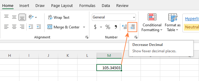
If you want to round numbers solely for presentations purposes, then you can just change the number of displayed decimal places without changing the underlying value. The fastest way is to use the Increase Decimal or Decrease Decimal command on the Home tab in the Number group:
Or you can change the cell's format by performing these steps:
- Select the cell with the number(s) you want to round.
- Open the Format Cells dialog by pressing Ctrl + 1 or right click the cell(s) and choose Format Cells... from the context menu.
- In the Format Cells window, switch to either Number or Currency tab, and type the number of decimal places you want to display in the Decimal places box. A preview of the rounded number will immediately show up under Sample.
- Click the OK button to save the changes and close the Format Cells dialog.

Important note! This method changes the display format without changing the actual value stored in a cell. If you refer to that cell in any formulas, the original non-round value will be used in all calculations.
Excel functions to round numbers
Unlike formatting options that change only the display value, Excel round functions alter the actual value in a cell.
Below you will find a list of functions specially designed for performing different types of rounding in Excel.
- ROUND - round the number to the specified number of digits.
- ROUNDUP - round the number upward to the specified number of digits.
- ROUNDDOWN - round the number downward to the specified number of digits.
- MROUND - rounds the number upward or downward to the specified multiple.
- FLOOR - round the number down to the specified multiple.
- CEILING - round the number up to the specified multiple.
- INT - round the number down to the nearest integer.
- TRUNC - truncate the number to a specified number of decimal places.
- EVEN - round the number up to the nearest even integer.
- ODD - round the number up to the nearest odd integer.
Excel ROUND function
ROUND is the major rounding function in Excel that rounds a numeric value to a specified number of digits.
Syntax: ROUND(number, num_digits)
Number - any real number you want to round. This can be a number, reference to a cell containing the number or a formula-driven value.
Num_digits - the number of digits to round the number to. You can supply a positive or negative value in this argument:
- If num_digits is greater than 0, the number is rounded to the specified number of decimal places.
For example
=ROUND(15.55,1)rounds 15.55 to 15.6. - If num_digits is less than 0, all decimal places are removed and the number is rounded to the left of the decimal point (to the nearest ten, hundred, thousand, etc.).
For example
=ROUND(15.55,-1)rounds 15.55 to the nearest 10 and returns 20 as the result. - If num_digits equals 0, the number is rounded to the nearest integer (no decimal places).
For example
=ROUND(15.55,0)rounds 15.55 to 16.
The Excel ROUND function follows the general math rules for rounding, where the number to the right of the rounding digit determines whether the number is rounded upwards or downwards.
Rounding digit is the last significant digit retained once the number is rounded, and it gets changed depending on whether the digit that follows it is greater or less than 5:
- If the digit to the right of the rounding digit is 0, 1, 2, 3, or 4, the rounding digit is not changed, and the number is said to be rounded down.
- If the rounding digit is followed by 5, 6, 7, 8, or 9, the rounding digit is increased by one, and the number is rounded up.
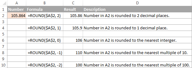
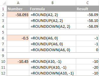
The following screenshot demonstrates a few ROUND formula examples:
Excel ROUNDUP function
The ROUNDUP function rounds the number upward (away from 0) to a specified number of digits.
Syntax: ROUNDUP(number, num_digits)
Number - the number to be rounded up.
Num_digits - the number of digits you want to round the number to. You can supply both positive and negative numbers in this argument, and it works like num_digits of the ROUND function discussed above, except that a number is always rounded upward.

Excel ROUNDDOWN function
The ROUNDDOWN function in Excel does the opposite of what ROUNDUP does, i.e. rounds a number down, toward zero.
Syntax: ROUNDDOWN(number, num_digits)
Number - the number to be rounded down.
Num_digits - the number of digits you want to round the number to. It works like the num_digits argument of the ROUND function, except that a number is always rounded downward.
The following screenshot demonstrates the ROUNDDOWN function in action.

Excel MROUND function
The MROUND function in Excel rounds a given number up or down to the specified multiple.
Syntax: MROUND(number, multiple)
Number - the value you want to round.
Multiple - the multiple to which you want to round the number.
For example, the below formula rounds 7 to the nearest multiple of 2 and returns 8 as the result:
=MROUND(7, 2)
Whether the last remaining digit is rounded up (away from 0) or down (towards 0) depends on the remainder from dividing the number argument by the multiple argument:
- If the remainder is equal to or greater than half the value of the multiple argument, Excel MROUND rounds the last digit up.
- If the remainder is less than half the value of the multiple argument, the last digit is rounded down.
The MROUND function comes in handy, say, for rounding prices to the nearest nickel (5 cents) or a dime (10 cents) to avoid dealing with pennies as change.

And, it is really indispensable when it comes to rounding times to a desired interval. For example, to round time to the nearest 5 or 10 minutes, just supply "0:05" or "0:10" for the multiple, like this:
=MROUND(A2,"0:05") or =MROUND(A2,"0:10")
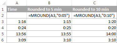
Note. The MROUND function returns the #NUM! error when its arguments have different signs. For example, both of the formulas =MROUND(3, -2) and =MROUND(-5, 2) result in the NUM error.
Excel FLOOR function
The FLOOR function in Excel is used to round a given number down, to the nearest multiple of a specified significance.
Syntax: FLOOR(number, significance)
Number - the number you want to round.
Significance - the multiple to which you wish to round the number.
For example, =FLOOR(2.5, 2) rounds 2.5 down to the nearest multiple of 2, which is 2.
The Excel FLOOR function performs rounding based on the following rules:
- If the number and significance arguments are positive, the number is rounded down, toward zero, as in rows 2 and 10 in the screenshot below.
- If number is positive and significance is negative, the FLOOR function returns the #NUM error, as in row 4.
- If number is negative and significance is positive, the value is rounded down, away from zero, as in row 6.
- If number and significance are negative, the number is rounded up, toward zero, as in row 8.
- If number is an exact multiple of the significance argument, no rounding takes place.
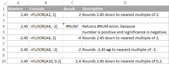
Note. In Excel 2003 & 2007, the number and significance arguments must have the same sign, either positive or negative, otherwise an error is returned. In newer Excel versions, the FLOOR function has been improved, so in Excel 2010, 2013 and 2016 it can handle a negative number and positive significance.
Excel CEILING function
The CEILING function in Excel rounds a given number up, to the nearest multiple of significance. It has the same syntax as the FLOOR function.
Syntax: CEILING(number, significance)
Number - the number you want to round.
Significance - the multiple to which you want to round the number.
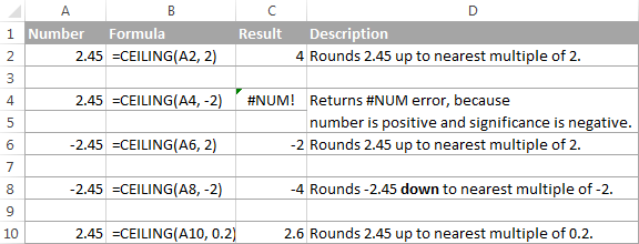
For instance, the formula =CEILING(2.5, 2) rounds 2.5 up to the nearest multiple of 2, which is 4.
The Excel CEILING function works based on the rounding rules similar to FLOOR's, except that it generally rounds up, away from 0.
- If both the number and significance arguments are positive, the number is rounded up, as in rows 2 and 10 in the screenshot below.
- If number is positive and significance is negative, the CEILING function returns the #NUM error, as in row 4.
- If number is negative and significance is positive, the value is rounded up, towards zero, as in row 6.
- If number and significance are negative, the value is rounded down, as in row 8.
Excel INT function
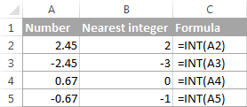
The INT function rounds a number down to the nearest integer.
Of all Excel round functions, INT is probably the easiest one to use, because it requires only one argument.
Syntax: INT(number)
Number - the number you want to round down to the nearest integer.
Positive numbers are rounded toward 0 while negative numbers are rounded away from 0. For example, =INT(1.5) returns 1 and =INT(-1.5) returns -2.
Excel TRUNC function
The TRUNC function truncates a given numeric value to a specified number of decimal places.
Syntax: TRUNC(number, [num_digits])
- Number - any real number that you want to truncate.
- Num_digits - an optional argument that defines the precision of the truncation, i.e. the number of decimal places to truncate the number to. If omitted, the number is truncated to an integer (zero decimal places).
The Excel TRUNC function adheres to the following rounding rules:
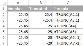
- If num_digits is positive, the number is truncated to the specified number of digits to the right of the decimal point.
- If num_digits is negative, the number is truncated to the specified number of digits to the left of the decimal point.
- If num_digits is 0 or omitted, it rounds the number to an integer. In this case, the TRUNC function works similarly to INT in that both return integers. However, TRUNC simply removes the factional part, while INT rounds a number down to the nearest integer.For example,
=TRUNC(-2.4)returns -2, while=INT(-2.4)returns -3 because it's the lower integer. For more info, please see Rounding to integer example.
The following screenshot demonstrates the TRUNC function in action:
Excel ODD and EVEN functions
These are two more functions provided by Excel for rounding a specified number to an integer.
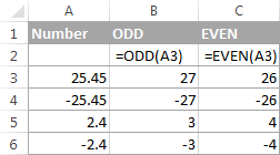
ODD(number) rounds up to the nearest odd integer.
EVEN(number) rounds up to the nearest even integer.
- In both functions, number is any real number that you want to round.
- If number is non-numeric, the functions return the #VALUE! error.
- If number is negative, it is rounded away from zero.
The ODD and EVEN functions may prove useful when you are processing items that come in pairs.
For example:
=ODD(2.4) returns 3
=ODD(-2.4) returns -3
=EVEN(2.4) returns 4
=EVEN(-2.4) returns -4
Using rounding formulas in Excel
As you see, there exist a variety of functions to round off numbers in Excel depending on the particular purpose. The following examples will hopefully give you some clues on how to use Excel rounding formulas based on your criteria.
How to round decimals in Excel to a certain number of places
Depending on the situation, you may want to round decimals up, down or based on math rounding rules:
ROUNDUP function - always rounds the decimal upward.
ROUNDDOWN function - always rounds the decimal downward.
ROUND - rounds up if the rounding digit is followed by the digit equal to or greater than 5, otherwise rounds down.
As an example, lets round the decimal numbers in column A to 2 decimal places. In the first argument (number), you enter a reference to the cell containing the number, and in the second argument (num_digits) you specify the number of decimal places you want to keep.
=ROUNDUP(A2, 2) - rounds the number in A2 upward, to two decimal places.
=ROUNDDOWN(A2, 2) - rounds the number in A2 downward, to two decimal places.
=ROUND(A2, 2) - rounds the number in A2 to 2 decimal places, upward or downward, depending on whether the 3rd decimal digit is greater or less than 5.

Rounding negative numbers (ROUND, ROUNDDOWN, ROUNDUP)
When it comes to rounding a negative number, the results returned by the Excel round functions, may seem to flout logic :)
When the ROUNDUP function applies to negative numbers, they are said to be rounded up, even though they actually decrease in value. For example, the result of =ROUNDUP(-0.5, 0) is -1, as in row 7 in the screenshot below.
The ROUNDDOWN function is known to round numbers downward, though negative numbers may increase in value. For example, the formula =ROUNDDOWN(-0.5, 0) returns 0, as in row 8 in the screenshot below.
In fact, the rounding logic with regard to negative numbers is very simple. Whenever you use the ROUND, ROUNDDOWN or ROUNDUP function in Excel on a negative number, that number is first converted to its absolute value (without the minus sign), then the rounding operation occurs, and then the negative sign is re-applied to the result.
How to extract a decimal part of a number
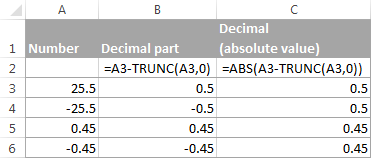
If you want to extract a fractional part of a decimal number, you can use the TRUNC function to truncate the decimal places and then subtract that integer from the original decimal number.
=A2 - TRUNC(A2,0)
As demonstrated in the screenshot below, the formula in column B works perfectly both for positive and negative numbers. However, if you'd rather get an absolute value (decimal part without the minus sign), then wrap the formula in the ABS function:
=ABS(A2 - TRUNC(A2,0))
How to round a decimal to an integer in Excel
As is the case with rounding to a certain number of decimal places, there is a handful of functions for rounding a fractional number to an integer.
ROUNDUP
To round up to nearest integer, use an Excel ROUNDUP formula with num_digits set to 0. For example =ROUNDUP(5.5, 0) rounds decimal 5.5 to 6.
INT or ROUNDDOW
To round down to nearest whole number, use either INT or ROUNDDOW with num_digits set to 0. For example both of the following formulas round 5.5 to 5:
=ROUNDOWN(5.5, 0)
=INT(5.5)
For negative decimals, however, the INT and ROUNDDOWN functions yield different results - INT rounds negative decimals away from 0, while ROUNDDOWN toward 0:
=ROUNDOWN(-5.5, 0) returns -5.
=INT(-5.5) returns -6.
TRUNC
To remove the factional part without changing the integer part, use the TRUNC formula with the second argument (num_digits) omitted or set to 0. For example, =TRUNC(5.5) truncates the decimal part (.5) and returns the integer part (5).
ODD or EVEN
To round a decimal up to the nearest odd integer, use the ODD function:
=ODD(5.5) returns 7.
To round a decimal up to the nearest even integer, use the EVEN function:
=EVEN(5.5) returns 6.

Round to nearest 0.5
Microsoft Excel provides 3 functions that let you round numbers to nearest half, more precisely to the nearest multiple of 0.5. Which one to use depends on your rounding criteria.
- To round a number down to nearest 0.5, use the FLOOR function, for example
=FLOOR(A2, 0.5). - To round a number up to nearest 0.5, use the CEILING function, for example
=CEILING(A2, 0.5). - To round a number up or down to nearest 0.5, use the MROUND function, e.g.
=MROUND(A2, 0.5). Whether MROUND rounds the number up or down depends on the remainder from dividing the number by multiple. If the remainder is equal to or greater than half the value of multiple, the number is rounded upward, otherwise downward.

As you see, the MROUND function can be used for rounding positive values only, when applied to negative numbers, it returns the #NUM error.
Round to nearest 5 / 10 / 100 / 1000
Rounding to nearest five, ten, hundred or thousand is done in the same manner as rounding to 0.5 discussed in the previous example.
Round to nearest 5
Supposing that the number you want to round to closest 5 resides in cell A2, you can use on of the following formulas:
- To round a number down to nearest 5:
=FLOOR(A2, 5) - To round a number up to nearest 5:
=CEILING(A2, 5) - To round a number up or down to nearest 5:
=MROUND(A2, 5)

Round to nearest 10
To round your numbers to nearest ten, supply 10 in the second argument of the rounding functions:
- To round a number down to nearest 10:
=FLOOR(A2, 10) - To round a number up to nearest 10:
=CEILING(A2, 10) - To round a number up or down to nearest 10:
=MROUND(A2, 10)

Round to nearest 100
Rounding to a hundred is done in the same way, except that you enter 100 in the second argument:
- To round a number down to nearest 100:
=FLOOR(A2, 100) - To round a number up to nearest 100:
=CEILING(A2, 100) - To round a number up or down to nearest 100
=MROUND(A2, 100)

Round to nearest 1000
To round a value in cell A2 to the nearest thousand, use of the following formulas:
- To round a number down to nearest 1000:
=FLOOR(A2, 1000) - To round a number up to nearest 1000:
=CEILING(A2, 1000) - To round a number up or down to nearest 1000
=MROUND(A2, 1000)

The same techniques can be used for rounding numbers to other multiples. For example, you can round the prices to the nearest nickel (multiple of 0.05), lengths to the nearest inch (multiple of 1/12), or minutes to the nearest second (multiple of 1/60). Speaking of time, and do you know how to convert it to nearest hour or closest 5 or 10 minutes? If you don't, you will find the answers in the next section :)
Rounding time in Excel
There may be many situations when you need to round time values. And again, you can use different rounding functions depending on your purpose.
Example 1. How to round time to nearest hour in Excel
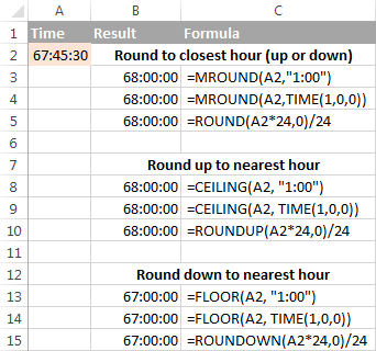
With times located in column A, you can use one of the following functions to round time to nearest hour:
- To round time to closest hour (up or down) - MROUND or ROUND.
=MROUND(A1,"1:00")=MROUND(A1, TIME(1,0,0))=ROUND(A1*24,0)/24 - To round up time to nearest hour - ROUNDUP or CEILING.
=CEILING(A1, "1:00")=CEILING(A1, TIME(1,0,0))=ROUNDUP(A1*24,0)/24 - To round down time to nearest hour - ROUNDDOWN or FLOOR.
=FLOOR(A1, "1:00")=FLOOR(A1, TIME(1,0,0))=ROUNDDOWN(A1*24,0)/24
In the ROUND, ROUNDUP and ROUNDDOWN formulas, you multiply the time value by 24 (number of hours in a day) to convert a serial number representing the time to hours. Then you use one of the rounding functions to round the decimal value to an integer, and then divide it by 24 to change the returned value back to the time format.
If your timestamps include date values, then use the INT or TRUNC function to extract dates (in the internal Excel system, dates and times are stored as serial numbers, the integer part representing a date and fractional part representing time). And then, use the formulas described above but subtract the date value. For example:
=MROUND(A1,"1:00") - INT(A1)
=MROUND(A1,"1:00") - TRUNC(A1)
The following screenshot demonstrates other formulas:
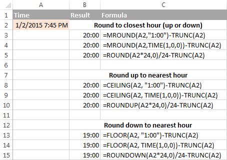
Note. For the results to display correctly, remember to apply the Time format to your cells.
Example 2. Rounding time to nearest 5, 10, 15, etc. minutes
In case you want to round times in your Excel sheet to five or ten minutes, or to the closest quarter-hour, you can use the same rounding techniques as demonstrated above, but replace "1 hour" with the desired number of minutes in the formulas.
For example, to round the time in A1 to the closest 10 minutes, use one of the following functions:
- To round time to closest 10 minutes (up or down):
=MROUND(A1,"0:10")=MROUND(A1, TIME(0,10,0)) - To round up time to nearest 10 min:
=CEILING(A1, "0:10")=CEILING(A1, TIME(0,10,0)) - To round down time to nearest 10 min:
=FLOOR(A1, "0:10")=FLOOR(A1, TIME(0,10,0))

If you know (or can calculate) what portion of a day is constituted by a certain number of minutes, then you won't have problems using the ROUND, ROUNDUP and ROUNDOWN functions as well.
For example, knowing that 15 minutes, is 1/96th of a day, you can use one of the following formulas to round the time in A1 to the nearest quarter-hour.
- To round time to closest 15 minutes (up or down):
=ROUND(A1*96,0)/96 - To round up time to nearest 15 min:
=ROUNDUP(A1*96,0)/96 - To round down time to nearest 15 min:
=ROUNDDOWN(A1*96,0)/96
This is how you perform rounding in Excel. Hopefully, now you know how, among all those round functions, chose the one best suited for your needs.
 by
by
368 comments
hi there!
im having a problem on how to put "if the tenths digit number is ODD;roundup and if the tenths digit number is EVEN;rounddown" in excel formula. thanks in advance!
example:
24.45= 24.4
24.15= 24.2
Hello,
Please try the following formula:
=IF(ISODD(MID(A1,FIND(".",A1)+1,1)),ROUNDUP(A1,1),ROUNDDOWN(A1,1))
Hope it will help you.
Hello,
I need a formula for below issue
12.45 = 12.45
12.23 = 12.23
12.51 = 13
12.79= 13
How can i round up number such as:
0.00 to 0.00
Below 0.01 to 0.00
above 0.01 to 1.00
how to 4165*10% round formula
Hi. I am trying to round the difference between 2 times to the nearest 15 min increment. I know I can use MROUND to round the times and then do the difference but trying to see if I can just do it on the difference. Thanks
Jay
After a few moments of play, I believe this accomplishes what I want.
{=SUM(ROUND(IF(ISNUMBER(A1:A5),A1:A5,0),0))}
Thank you for this site, which got me thinking about a solution.
When summing rounded values, as in:
{=SUM(ROUND(A1:A5,0))}
some cells may not contain a number value (common case as in "N/A").
Any thoughts whether it is possible to add validation as number prior to the round function, so that the formula does not return #VALUE!? Essentially, eliminate non-numeric values, before rounding each, and then summing.
Hello,
Thank you for the helpful information. I just wanted to point out that under the "TRUNC Function", in the screenshot example, the third row's formula should be "=TRUNC(A3,1)" in order to get the number in B3. Just don't want others to get confused.
Thanks,
Steven
Hello Steven,
Thank you for pointing that out! Fixed.
Hi,
Is there a way to round up an input in the same cell without adding a new column for the return result? eg, data validation?
I want to know the formula which decimals not to calculate while sum total
if
1.5 1.5 1.5 1.5 1.5 1.5 --> 6 to calculate with out decimal caculateing
Hey, does anyone know how I can round up or round down an equation?
(A1-10)/2
=ROUND((A1-10)/2,0)
The 0 is for no decimal places. replace it with 2 for 2 decimal places or maybe with -1 to round to the nearest 10.
Hi,
is there anybody who knows how I can round the calculation result to end in -9
I have a forumula (D2 + $H$2 +$H$4 + $H$5)the result of which i want to end in number -9
bgrds
Dodo
Hello, how do i formulate a cell for the figures to end in a certain number (ex. 195, 295) and not in multiples of 95?
Hello, I want to roundup cell 2564 =2560 and I want to roundup the 2564 =2570 in same cell and How can I do this task.
I need to Round the following lines to the nearest 1/16. But Excel will not allow this. for example,
IF(D9=2,D5/2,
I may get 83.3333 but I need 83.125.
=IF(OR(D3=0,D3=""),"",
IF(D9=1,D5,
IF(D9=2,D5/2,
IF(D9=3,D5/3,
IF(D9=4,D5/4,
IF(D9=5,D5/5,
IF(D9=6,D5/6,
IF(D9=7,D5/7,""))))))))
I am needing to found any thing above 100 back down to 100. How do I write this formula?
Hi,
Which formula used for the round in the multiple of 10 for both figure( Negative as well as positive).
Mround is used only for the positive figure and rounddown is for negative figure but i want 1 formula for both the figure.
Is there any???
Please tell me............
Hullo, I want to roundup cell I3 which carries an amount 2100 and I want to roundup the same as 3,000 in another cell and How can I do this task.
whole numbers such as 201
202
203
204
205
206
207
208
290
210
1-2 round down ie 201 to 199 202 to 199
3-6 rounded to 5
202 203 204 205 206 become 205
207 208 209 210 become 209
anyone help?
Good afternoon,
I'm needing to add 2 different percentages to a formula and they both need to round. I will need to round the first percentage before i can add the second percentage to that number. Right now excel will not allow me to round each percentage but will allow me to round both percentages at the end.
example:
this is what i need to happen in my formula
218*-15%= -32.7 (round up)
218-33=185
185*8%=14.8 (round up)
185+15=200
200+205=405
405 is the number i need to reach
and this is my formula in excel now:
A3=218
B3=-15%
C3=8%
D3=205
=ROUND(A3*B3+A3*C3,0)+A3+D3 and that comes up to 408, which is 3 over from 405
Before, i needed to only add one percentage and the round formula works great but i cannot find a way to get it close. I have tried with a larger number, replace A3(218) with 1304 and the gap was larger and will cause problems.
example:
it should figure out to 1402
1304*-15%=195.6 (round up)
1304-196=1108
1108*8%=88.64 (round up)
1108+89=1197
1197+205=1402
And in excel, with the same formula as above, i get 1418. I know with percentages you will have numbers be maybe 1 or 2 off due to rounding but this is too great and will not work.
Please let me know if there is another way to write this formula to make it work properly.
Thanks.
well i found a formula that worked
(ROUND((8%+1)*(ROUND(218*-15%,0)+218),0))+205=405
just fyi...
Hi, Can hi you help me to get this?
I can't really came up with a solution for this problem
say I want 1mins-4mins rounded into 0 and 5mins-19mins rounded into 15mins then 20-34mins rounded into 30mins and 35mins-1hr4mins rounded into 1hr/60mins
i hope yo ucan help me with this thanks :)
Please help me get the rounddown or roundup for the following:
a) 1.01 - 1.85 round down to 1
b) more than 1.86 round up to 2
=ROUND(B1/10^TRUNC(LOG(B1)),A1-IF(B1>1,1,0))*10^TRUNC(LOG(B1))
I prematurely posted a significant digit rounding I've been using. Sediment is what I deal with and it is the size of clay in mm to cobble in mm, where significant digits count. I don't know of a function to do this so I wrote this formula; =ROUND(B1/10^TRUNC(LOG(B1)),A1-IF(B1>1,1,0))*10^TRUNC(LOG(B1)) with cell A1 the significant digits and B1 the input number to be rounded.
Hi Team,
I want a simple formula for round-off, like -
a) 0 Years, 9 Months, 15 Days - Should be rounded off to 9 Months
b) 0 Years, 9 Months, 16 Days - Should be rounded off to 10 Months
means, anyone, below 15 or equivalent to 15 days would remain 09 Months and
anyone, greater than or equivalent to 16 days would be 10 months.
Thanks & regards
Arnab Sarkar
In cell A1 have 10 and cell B1 is 8.50681, when I multiply A1*B1 result appear is "85.0681", But I show in Cell B1 is 8.50 till (2 decimal point). And now I want to multiply A1*B1, and I want that excel count till 2 decimal point like 8.50 in B1. Is it possible? remember B1 actual value is 8.50681.
what i have to do if bulk amount need to round off, if the amount will >5 so it will grow upside,if the amount <5 so it will get down side
How to convert upper than 15 digit value in excel
I am having a problem using ceiling function.
Now my Problem is : I want to ceil few values upto 0.5 and then rest upto 0.25 in the SAME CELL !! like if i want to ceil values between 2 and 3 upto 0.5 i.e if i write 2.3 it gives me 2.5 or if i write 2.74 it gives me 3. But in the same cell if i write values between 0.5 to 2, it should ceil me upto 0.25 i.e. if i write 1.2 it should give me 1.25 or if i write 1.67 it should give me 1.75. Hoping for a reply. Thanks for the concern.
Can you explain why this happens?
For the same input of 0.01, the spreadsheet should not be giving .02, .02 is incorrect. But why? Thanks.
=ceiling(0.01,0.01) = .01
=ceiling(16.00-15.99,0.01) = .01
=ceiling(16.01-16.00,0.01) = .02
=roundup(0.01,2) = .01
=roundup(16.00-15.99,2) = .01
=roundup(16.01-16.00,2) = .02
can I round up years? for example 1 years, 3 months, 4 days, rounded up to 2 years.
Could you give me the formulation? thanks.
Is there a way to force excel to round the following decimal down, instead of up? $2.225. I want it to round any number where the third decimal place is a "5" (and only a 5, not any other number) down, instead of up.
For instance: $2.225 to $2.22
$2.226 auto rounds to $2.23, this is fine
$2.224 auto rounds to $2.22, this is fine
Is there any way to round a column of currency to an even number (reducing a dollar amount by $.01)
$887.65 to $887.64 leaving the even numbers as is.
I can easily round up. I'm not finding a way to round down.
Hi Julie,
To round down to the even hundredth, you can use the FLOOR function with multiple 0.02, e.g.:
=FLOOR(A1, 0.02)
maam, how to round off even a minute to the next(higher hour) ex.01:05 to 02:00 hrs please help
0
Hi Kandan,
You can use any of the following formulas:
=CEILING(A1, TIME(1,0,0))
=CEILING(A1, "1:00")
=ROUNDUP(A1*24,0)/24
Hi, I want round off this time,1:16 to the nearest 5 minutes,anybody can help me
Hi Masooda,
To round time to the nearest 5 minutes, you can use the MROUND function with multiple equal to "0:05", e.g.:
=MROUND(A1,"0:05")
Can you explain why this happens?
=ceiling(0.01,0.01) = .01
=ceiling(16.00-15.99,0.01) = .01
=ceiling(16.01-16.00,0.01) = .02
=roundup(0.01,2) = .01
=roundup(16.00-15.99,2) = .01
=roundup(16.01-16.00,2) = .02
Hey - I wondered if you might help. I'm trying to work on membership rates and wanting to round down to $1,500 if the formula we use surpasses that mark. Any ideas people? Many thanks in advance.
Hi Richard,
You can embed your formula into the IF function, like this:
=IF(formula()>1500, 1500, formula())
if i have a function that if c1=8 and c1 cells contains value 8 and then i create this that if the value is true then i will forward that if it is true then it take the value of cell d1 which value is 2x1.8 then how i will solve this that it gives value 3.6 automatically not the value same 2x1.8 in the cell where i put this formula
if i have a function that if c1=8 and c1 cells contains value 2x1.8 then how i will solve this that it gives value 3.6 automatically not the value same 2x1.8 in the cell where i put this formula
Very helpful it was required while working and finally I got the solution and the result...
Thank you...
Hi
Firstly great article very useful info on rounding.
Now to my query is there a formula that will convert negative figures into positive figures with out affecting the value.
The reason for this is I'm a bookkeeper and when i am downloading reports to excel to match to data downloaded from a CV file from bank. The debit side will sometimes show in a negative dependant on program its downloaded from, its makes it a nuisance when it in a negative as I have to add the figures together as one report will have positive figures and other report will have negative figure. When I would rather just do the usual (this-this=this), the outcome its to have the amount it equals to is 0. Then we know our reports match, & if it doesn't it then helps us find the out of balance amount.
If we add further information to get a percentage or divided value, if the amount is in negative it gives an incorrect figure. Going through every figure and removing the - from the each amount takes up a lot of time, especially when the report is very long. This is time wasted when i could be making use of my time more efficiently.
Im hoping yo will say yep here is an easy fix and not say no sorry no solution. My fingers are crossed
Regards Vivien Anderson
C/- VLA Bookkeeping Services
=(G54-F54)/(K54/L54)*2 = 11013.1765 round
=(G54-F54)/(K54/L54)*2 PLS ROUND UP THIS FORRMULATION
Good day. How can i round up number such as:
0.00 to 0.00
0.01 to 0.00
0.02 to 0.00
0.03 to 0.00
0.04 to 0.05
0.05 to 0.05
0.06 to 0.05
0.07 to 0.10
0.08 to 0.10
0.09 to 0.10
0.10 to 0.10
Hi, please can someone help. I need to round my pricing so that the numbers end in either a 5 or a 9. The prices are whole numbers without decimals e.g $893.
The rules are as follows
Number ending:
1 - round down to 9
2 - round up to 5
3 - round up to 5
4 - round up to 5
5 - no change
6 - round down to 5
7 - round up to 9
8 - round up to 9
9 - no change
0 - round down to 9
can any one solve this issue
any numeric number convert in to number like
<3 = 0
3=3
4=3
5=3
6=6
7=6
8=6
9=9
10=9
Is there any way to set a rule in terms of when to round?
For instance, at my job when we're billing by hand, we round anything 0.456 or above to 1 and anything 0.455 or below to 0. In Excel, however, I've tried several different ways to round according to the rules of my job with no luck. 0.456, even 0.5 most of the time, gets rounded down to 0. We create these number charts and most numbers round correctly but some numbers do fall victim to this discrepancy and I need to make sure we don't have errors because of this issue. What do you suggest?
Hello,
I am trying to sum multiple decimals. If sum equals .05 or higher, I need to round up to the nearest whole number. Here is an example:
0.47
0.19
0.39
-------
1.05
I need to round up to 2.00
If sum equals 2.07 round up to 3.00 etc..
Thanks for your time!
Jason
Hello,
I am trying to sum multiple decimals. If sum equals .05 or higher, I need to round up to the nearest whole number. Here is an example:
0.47
0.19
0.39
-------
1.05
I need to round up to 2.
If sum equals 2.07 round up to 3 etc..
Thanks for your time!
Jason
hi,
Anybody can tells me. how i can count such below within a one Drag.
1 to 5 = count as 5
6 to 10 = count as 10
11 to 20 = count as 20
Thanks
Kuldeep Singh
Mob:- 9540790777
Hello Kuldeep,
Please try this formula:
=IF(AND(1 <=C18,C18<=5), 5,0)+IF(AND(6 <=C18,C18<=10), 10,0)+IF(AND(11 <=C18,C18<=20), 20,0)
Hi, Fedor, Can you help with my formula, which I think is similar to the problem above. I need to round my pricing so that the numbers end in either a 5 or a 9. The prices are whole numbers without decimals e.g $893.
The rules are as follows
Number ending:
1 - round down to 9
2 - round up to 5
3 - round up to 5
4 - round up to 5
5 - no change
6 - round down to 5
7 - round up to 9
8 - round up to 9
9 - no change
0 - round down to 9
HI THIS NOT WORKING PLEASE SEND ME AGAIN THIS IS VERY IMPORTAND TO ME
=ROUND(SUM(B5*(113/113)+64.5-71),0)
If anyone can help me with the above formula.
With the above the positive numbers are moved away from zero to the next whole number and negative numbers are also moved away from zero to the next whole number.
Examples (Positive) :
1.6=2
1.5=2
1.4=1
Examples (Negative)
-1.6=-2
-1.5=-2
-1.4=-1
The positive numbers are fine the fix I am looking for is when the negative numbers finish in -0.5 they get moved away from zero to the next whole number but I need them to go towards zero as shown in the examples below.
Examples (Negative)
-0.5=0
-1.5=-1
-2.5=-2
So the function I am looking for is to move positive numbers away from zero, and negative numbers towards zero when they finish either 0.5 or -0.5 to the next whole number
Hope you can help
Regards Keith
Hello Keith,
Please try this formula: =TRUNC(L5, 0)+IF(L5-TRUNC(L5) >= 0.5, 1, 0)
You should get the following result:
1.6 2
1.5 2
1.4 1
-0.5 0
-1.5 -1
-2.5 -2
CAN YOU HELP ME TO GET THE FOLLOWING RESULT? ANY FORMULA FOR THIS?
0 TO 0.3= 0
0.31 TO .80=.5
0.81 TO 1= 1
Thank u for your guidance
Regards
I want to make grade of a exam result sheet. Grades will be if marks between 50 and 54, "C", Marks bet. 54 and 60, "B", bet. 60 and 100, "A". Please show How do I have to write the formula?
Hello Ckandana,
You can use a nested IF formula like in the following example:
Using multiple IF functions in Excel