In this article, you will find two quick ways to change the background color of cells based on value in Excel 2016, 2013 and 2010. Also, you will learn how to use Excel formulas to change the color of blank cells or cells with formula errors.
Everyone knows that changing the background color of a single cell or a range of data in Excel is easy as clicking the Fill color ![]() button . But what if you want to change the background color of all cells with a certain value? Moreover, what if you want the background color to change automatically along with the cell value's changes? Further in this article you will find answers to these questions and learn a couple of useful tips that will help you choose the right method for each particular task.
button . But what if you want to change the background color of all cells with a certain value? Moreover, what if you want the background color to change automatically along with the cell value's changes? Further in this article you will find answers to these questions and learn a couple of useful tips that will help you choose the right method for each particular task.
How to change a cell's color based on value in Excel dynamically
The background color will change dependent on the cell's value.
Task: You have a table or range of data, and you want to change the background color of cells based on cell values. Also, you want the color to change dynamically reflecting the data changes.
Solution: You need to use Excel conditional formatting to highlight the values greater than X, less than Y or between X and Y.
Suppose you have a list of gasoline prices in different states and you want the prices greater than USD 3.7 to be of the color red and equal to or less than USD 3.45 to be of the color green.
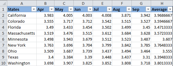
Note: The screenshots for this example were captured in Excel 2010, however the buttons, dialogs and settings are the same or nearly the same in Excel 2016 and Excel 2013.
Okay, here is what you do step-by-step:
- Select the table or range where you want to change the background color of cells. In this example, we've selected $B$2:$H$10 (the column names and the first column listing the state names are excluded from the selection).
- Navigate to the Home tab, Styles group, and choose Conditional Formatting > New Rule….

- In the New Formatting Rule dialog box, select "Format only cells that contain" under "Select a Rule Type" box in the upper part of the dialog box.
- In the lower part of the dialog box under "Format Only Cells with section", set the rule conditions. We choose to format only cells with a Cell Value - greater than - 3.7, as you can see in the screenshot below.
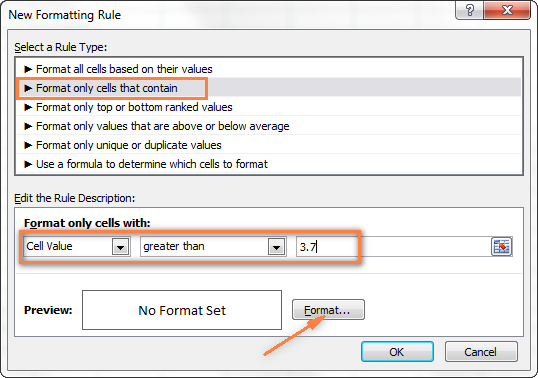
Then click the Format… button to choose what background color to apply when the above condition is met.
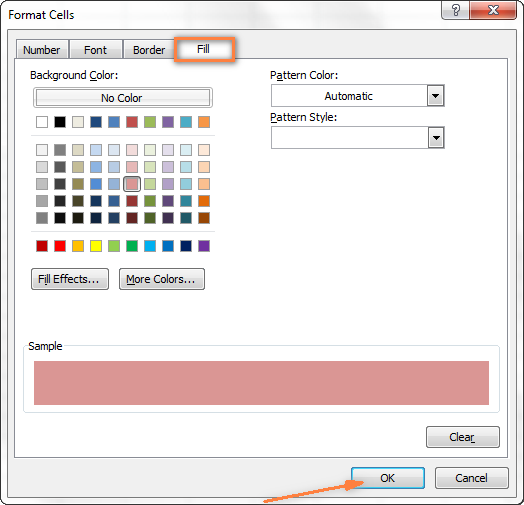
- In the Format Cells dialog box, switch to the Fill tab and select the color of your choice, the reddish color in our case, and click OK.
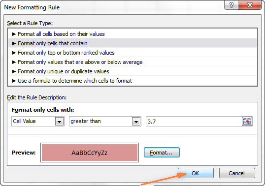
- Now you are back to the New Formatting Rule window and the preview of your format changes is displayed in the Preview box. If everything is Okay, click the OK button.
The result of your formatting will look similar to this:
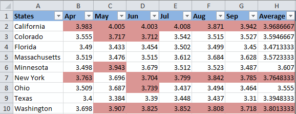
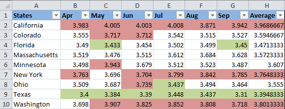
Since we need to apply one more condition, i.e. change the background of cells with values equal to or less than 3.45 to the green color, click the New Rule button again and repeat steps 3 - 6 setting the required condition. Here is the Preview of our second conditional formatting rule:

When you are done, click the OK button. What you have now is a nicely formatted table that lets you see the highest and lowest gas prices across different states at a glance. Lucky they are in Texas :)
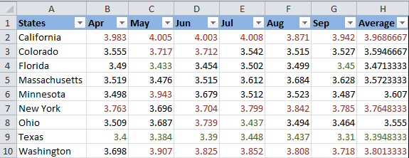
Tip: You can use the same method to change the font color based on the cell's value. To do this, simply switch to the Font tab in the Format Cells dialog box that we discussed in step 5 and choose your preferred font color.
How to permanently change a cell's color based on its current value
Once set, the background color will not change no matter how the cell's contents might change in the future.
Task: You want to color a cell based on its current value and wish the background color to remain the same even when the cell value's changes.
Solution: Find all cells with a certain value or values using Excel's Find All function or Select Special Cells add-in, and then change the format of found cells using the Format Cells feature.
This is one of those rare tasks that are not covered in Excel help files, forums and blogs and for which there is no straightforward solution. And this is understandable, because this task is not typical. And still, if you need to change the background color of cells statically i.e. once and forever unless you change it manually again, proceed with the following steps.
Find and select all cells that meet a certain condition
There may be several possible scenarios depending on what kind of values you are looking for.
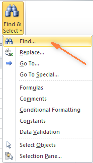
If you need to color cells with a particular value, e.g. 50, 100 or 3.4, go to the Home tab, Editing group, and click Find Select > Find….
Enter the needed values and click the Find All button.
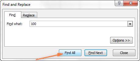
Tip: Click the Options button in the right-hand part of the Find and Replace dialog to get a number of advanced search options, such as "Match Case" and "Match entire cell content". You can use wildcard characters, such as an asterisk (*) to find any string of characters or a question mark (?) to find any single character.
In our previous example, if we needed to find all gas prices between 3.7 and 3.799, we would specify the following search criteria:
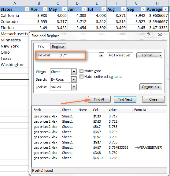
Now select any of the found items in the lower part of the Find and Replace dialog window by clicking on it and then press Ctrl + A to select all found entries. After that click the Close button.
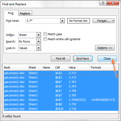
This is how you select all cells with a certain value(s) using the Find All function in Excel.
However, what we actually need is to find all gas prices higher than 3.7 and regrettably Excel's Find and Replace dialog does not allow for such things.
Luckily, there is another tool that can handle such complex conditions. The Select Special Cells add-in lets you find all values in a specified range, e.g. between -1 and 45, get the maximum / minimum value in a column, row or range, find cells by font color, fill color and much more.
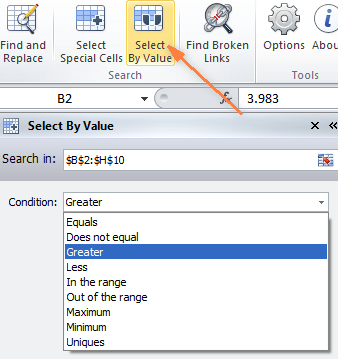
You click the Select by Value button on the ribbon and then specify your search criteria on the add-in's pane, in our example we are looking for values greater than 3.7. Click the Select button and in a second you will have a result like this:
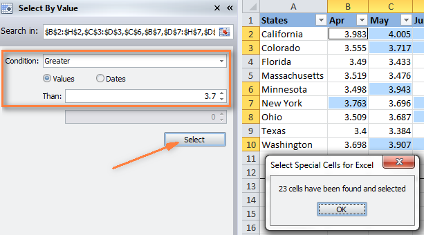
If you are interested to try the Select Special Cells add-in, you can download an evaluation version here.
Change the background color of selected cells using "Format Cells" dialog
Now that all cells with a specified value or values are selected (either by using Excel's Find and Replace or Select Special Cells add-in) what is left for you to do is force the background color of selected cells to change when a value changes.
Open the Format Cells dialog by pressing Ctrl + 1 (you can also right click any of selected cells and choose "Format Cells…" from the pop-up menu, or go to Home tab > Cells group > Format > Format Cells…) and make all format changes you want. We will choose to change the background color in orange this time, just for a change :)
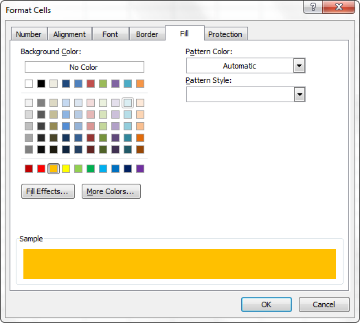
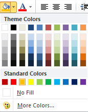
If you want to alter the background color only without any other format changes, then you can simply click the Fill color button and choose the color to your liking.
Here is the result of our format changes in Excel:
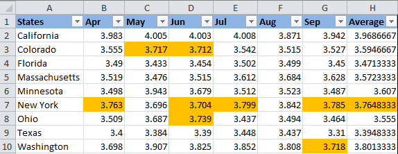
Unlike the previous technique with conditional formatting, the background color set in this way will never change again without your notice, no matter how the values change.
Change background color for special cells (blanks, with formula errors)
Like in the previous example, you can change the background color of special cells in two ways, dynamically and statically.
Use Excel formula to change background color of special cells
A cell's color will change automatically based on the cell's value.
This method provides a solution that you will most likely need in 99% of cases, i.e. the background color of cells will change according to the conditions you set.
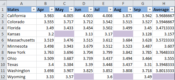
We are going to use the gas prices table again as an example, but this time a couple of more states are included and some cells are empty. See how you can detect those blank cells and change their background color.
- On the Home tab, in the Styles group, click Conditional Formatting > New Rule… (see step 2 of How to dynamically change a cell color based on value for step-by-step guidance).
- In the "New Formatting Rule" dialog, select the option "Use a formula to determine which cells to format". Then enter one of the following formulas in the "Format values where this formula is true" field:
- =IsBlank()- to change the background color of blank cells.
- =IsError() - to change the background color of cells with formulas that return errors.
Since we are interested in changing the color of empty cells, enter the formula =IsBlank(), then place the cursor between parentheses and click the Collapse Dialog button
 in the right-hand part of the window to select a range of cells, or you can type the range manually, e.g.
 =IsBlank(B2:H12).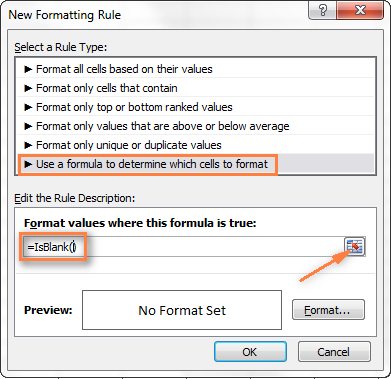
- Click the Format… button and choose the needed background color on the Fill tab (for detailed instructions, see step 5 of "How to dynamically change a cell color based on value") and then click OK.
The preview of your conditional formatting rule will look similar to this:

- If you are happy with the color, click the OK button and you'll see the changes immediately applied to your table.
Change the background color of special cells statically
Once changed, the background color will remain the same, regardless of the cell values' changes.
If you want to change the color of blank cells or cells with formula errors permanently, follow this way.
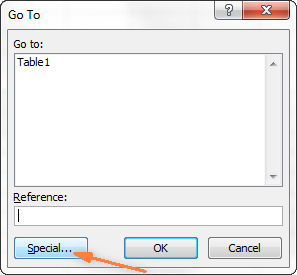
- Select your table or a range and press F5 to open the "Go To" dialog, and then click the "Special…" button.
- In the "Go to Special" dialog box, check the Blanks radio button to select all empty cells.
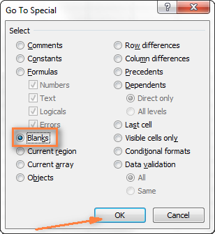
If you want to highlight cells containing formulas with errors, choose Formulas > Errors. As you can see in the screenshot above, a handful of other options are available to you.
- And finally, change the background of selected cells, or make any other format customizations using the "Format Cells" dialog as described in Changing the background of selected cells.
Just remember that formatting changes made in this way will persist even if your blank cells get filled with data or formula errors are corrected. Of course, it's hard to imagine off the top of the head why someone may want to have it this way, may be just for historical purposes :)
How to get most of Excel and make challenging tasks easy
As an active user of Microsoft Excel, you know that it has plenty of features. Some of them we know and love, others are a complete mystery for an average user and various blogs, including this one, are trying to shed at least some light on them. But! There are a few very common tasks that all of us have to perform daily and Excel simply does not provide any features or tools to automate them or make an inch easier.
For example, if you need to check 2 worksheets for duplicates or merge rows from single or different spreadsheets, it would take a bunch of arcane formulas or macros and still there is no guarantee you would get the accurate results.
That was the reason why a team of our best Excel developers designed and created 70+ add-ins that we call the Ultimate Suite for Excel. These smart tools handle the most grueling, painstaking and error-prone tasks in Excel and ensure quickly, neatly and flawless results. Below is a short list of just some of the tasks the add-ins can help you with:
- Remove duplicates and find unique values
- Merge tables and combine data from different sources
- Combine duplicate rows into one
- Merge cells, rows and columns
- Find and replacing in all data, in all workbooks
- Generate random numbers, passwords and custom lists
- And much, much more.
Just try these add-ins and you will see that your Excel productivity will increase up to 50%, at the very least!
That's all for now. In my next article we will continue to explore this topic further and you will see how you can quickly change the background color of a row based on a cell value. Hope to see you on our blog next week!
 by
by
424 comments
Hello,
I need to create a rule where if one cell contains specific text ('Yes'), it highlights in one colour (yellow) and then if another 'Yes' is present in the cell next to it (same row), then the second 'Yes' cell will turn Orange and the red for a third 'Yes'.
Is this possible?
Or - (for example) if C1 contains 'Yes', then a A1 and B1 turns yellow, and if D1 also contains a 'Yes', the A1 and B1 turns orange and so on.
Thank you in advance!!
I would like to format one of the columns in my spreadsheet to highlight if there is a value present in another column. What I am trying to do is show whether materials are present or not and I would like to show an indicator in one of my first columns.
Thank you!
Hello, Desiree,
you need to use conditional formatting based on another cell value. Please take a look at this article of ours. If you pay attention and follow the steps, you'll manage to solve your task :)
thnx for all of these
Hi,
I want to change 15 cell colour if another cell is blank(no value).
I tried by using condition format " format only cell contain", but it some time it working and some time not working.
Please help me to fix issue.
Hi Excel novice here.
I need a cell to change colour if the total of a column is between 2 numbers. How would I go about doing that?
Hi, Gavin,
here are a few articles for you to check out in order to solve the problem:
1) these basic formulas and functions will give you a great understanding of the logic of all the Excel operations and calculations - will help to set the right criteria (if the total is between two numbers)
2) conditionally formatted rule will colour the cells depending on some criterion
3) here are the ways of building formulas to sum the values
I do hope that you'll take a look at this great and easy tutorials and will be able to solve your task :)
thank you
Hi Svetlana Cheusheva,
Thank you so much,
your article is really helpful.
I have problem that,
How to add "Ablebits" option?
Greetings,
I want to highlight a row in the following manner:
1. Columns C, D, and E will have an X entered in them and they are for good, not good, partially good.
2. When I put an X in the good column for that row, I would like the row from columns A through J to highlight Green, Not good = Red, partially good = yellow. If there is no X in either 3 of these columns then the row is blue. If all 3 have an X then it should also turn Red.
Is there any possible way this could be done through excel?
Thanks in advance.
hi.. Please tell me if i have a huge data and there is some coloured cell so how can i copied or filtered only those cell which are coloured.
How to change the color of States column (column A) automatically according to the color of conditional format applied in other column (Column B)?
thanks i problem solved
Hi use this site as I am just more than a novice with Excel but this helps me set what appear to be impossible tasks with ease, all explained in laymans terms.
Many Thanks
Malcolm
Hi,
I've a array of data (600 rows X 300 columns) want to compare 2 rows of data with conditional formatting and change color. The problem I facing is I can't able to write formula for each cell. If u know any special formula which can be used for entire array, kindly us know.
For Eg, Compare A1 & A2 if A2 is less than A1, change color. Similar need to do for A3&A4, A5&A6, B1&B2, B3&B4, B5&B6, C1&C2, C3&C4, etc...
Don't why below scenario did not post...seeking auto solution
B3 is red if less than B2
B3 is green if greater the B2
B4 is red if less than B3
B4 is green if grater than B3
ect...
Hi,
yet, I don't example for :
easy coloring backgroud of cells for chosen values in cells
For example in the row I have values 0 - 100 - in 101 columns
I chose values : e.g. 37, 56, 100 and I want these cells
with chosen backgroud color. For example green.
Thank you for help
Hi,
Is there a way to format the cells to change from one colour to another depending on a word added to the cell. I want to add "anyword" meaning any word added to the cell will change the colour of the cell.
Thanks,
Practical.
thank you.
If the Cell A1 is Colour than its - 1
If the cell A1 is Blank than its - 2
hi,
Need Your help..
I have problem of high light lowest value from diff.Columns in single row
e.g. i want to do find lowest value from e6:h6 and then highlight with red colur & bold it.
Is it possible to fill up text for the value of cell?? Means if the value of cell is 100, it format text as "Below average". Is it possible?
Thank you very much.....................
Hi Svetlana Cheusheva,
How the color of the cell will be changed automatically to the same color of a cell already changed via conditional formatting?
Great, Great,Great..
Very useful article.
i got much help from here.
Thanks alot..
I want to change the color of a cell on one tab and have it automatically change the color of a cell on a different tab. How can I do this? Both cells will have the same text, but be in a different place. I know how to copy data from one sheet to another. But I don't know how to copy the cell color too.
Congratz. This is very helpful.
Dear Svetlana cheusheva
I need an formula for changing the background color in Excel sheet if the value changes then the color of background automatically change using excel formula .Kindly revert if any information required
Dear Svetlana cheusheva
I need an formula for changing the background color in Excel sheet if the value changes then the color of background automatically change using excel formula .Kindly revert if any any information required
Hi SC,
This article is really helpful.
I just want to know
Is it Possible to change the color of the text in this way?
Hello Ali,
Of course, it's possible. When setting the format, switch to the Font tab instead of the Fill tab, and select the font color you want.
I want color in cell according to value as like tank level indication
Thank you so much... It helped me a lot. I got a great applause from my team. thank you... :) :) :)
Hi
Could you please advise? How cell will be auto highlighted if we will do any amendment.
i have raw data and values are there but in order to make a report i need to change some values. But after that report i want original data. So if there will be auto highlighted function then i can see the cell easily and put the original value back.
Looking for your urgent reply.
Thank you
Why not keep a master copy of your document and then work only on a copy, so that changes to the copy don't make change to the master document?
Hi Svetlana,
Thanks for wondering excel formatting techniques. I would like to know about colour change in excel formatting, When a cell colour is already coloured by conditional formatting, when task changes, i want the colour of that cell to be changed. Could you please give some ideas to that.
thks in advance
rahul
How to add 4rth condition as i want to make 4 conditions for a cell to change color
Hey ,
Can some one help to achieve this task :
I need to change color of A1 cell based upon following criteria .
if Cell A2 to A10 value is = Y
then
color of A1 cell will be Red
Else
color of A1 cell will be Green
thanks a lot
thanks alot, for the information
Hey,
I want excel to change the color of cell in one sheet when value of it's reference cell has been changed in another sheet.
e.g.
sheet 2 contains values referred from sheet 1
and sheet 2 is completely protected.
Then any value in particular cell modified in Sheet 1 shall displayed with another background color in protected Sheet 2
Please let me know, if its possible.
Thanks.
I have B1 through B400 that I need each cell to change based on cell A1 through A400. I do not want to format each cell manually. Copy and past has all the B cells referance A1. What am I doing wrong?
I have two coloum in excel one order qnt and obe export qnt and I want after full qnt export automatic course change of qnt.
Dear sevetlana,
Tell me can i put sell value according to name like 'open'and 'closed'.
and if yes then how.
Ajay
Finally some easy to follow steps. I needs this time to time and I'm often struggling to achiev what I wanted. This one was awesome ;-)
clear n precise...very very useful
Thanks a ton
Hi Everybody,
I need your help.I wanna to fill colour only numeric in excel.
Number is 10000 between 20000.This numbers are fill colour after choice.
Thus, If it's not ok.
Give me another one method, and how to write macro.
Please explain me!
I need to change the colour of cell as follows
A B C
1 38 40
2 38 42
3 38 35
If B1 is greater than or equal to A1 the colour of C1 should be green otherwise it should be red. Pls help
Thank you very much.
This Article is very helpful and it contains many solutions for excel.
Am prepare timeline chart for project. i need to highlight sundays dates.how to color Sundays by conditional format
I have 2 column's one for start date and the other end date - and next coloum gives the numbers of days between the start date and end date ..
if i say
Column E -- start date
Column F -- End Date
Column G -- no of days
If i want to get the cells in Coloumn G coloured for all the row which donot have a end date ..... how can I format it .
This is awesome, thank you.
I am wondering: I have a group of cells in which I have numbers, and I am usin the MIN command to find the lowest number between these cells. I would like to have a cell next to the one displaying the lowest number then display a block of text and a cell color based on which of these cells has the lowest number, so I can basically show a "winner" of which number is the lowest in the data set. Is this possible?
So essentially it looks like:
1 2 3
Thank you!
I would like to conditionally format cells that contains a date, based on values in different cells. My cell contains a date (indicates due date) and the gradient bar behind it would indicate percentage complete in color (stored in a different cell). Can you provide some help please?
I want line charts details ,with green colour line shows if its upward and red colour line shows if its Downward ,one line in one chart