This tutorial focuses on various ways to calculate times in Excel. You will find a few useful formulas to add and subtract times, calculate time difference, or elapsed time, and more.
In the last week's article, we had a close look at the specificities of Excel time format and capabilities of basic time functions. Today, we are going to dive deeper into Excel time calculations and you will learn a few more formulas to efficiently manipulate times in your worksheets.
How to calculate time difference in Excel (elapsed time)
To begin with, let's see how you can quickly calculate elapsed time in Excel, i.e. find the difference between a beginning time and an ending time. And as is often the case, there is more than one formula to perform time calculations. Which one to choose depends on your dataset and exactly what result you are trying to achieve. So, let's run through all methods, one at a time.
Formula 1. Subtract one time from the other
As you probably know, times in Excel are usual decimal numbers formatted to look like times. And because they are numbers, you can add and subtract times just as any other numerical values.
The simplest and most obvious Excel formula to calculate time difference is this:
Depending on you data structure, the actual time difference formula may take various shapes, for example:
| Formula | Explanation |
=A2-B2 |
Calculates the difference between the time values in cells A2 and B2. |
=TIMEVALUE("8:30 PM") - TIMEVALUE("6:40 AM") |
Calculates the difference between the specified times. |
=TIME(HOUR(A2), MINUTE(A2), SECOND(A2)) - TIME(HOUR(B2), MINUTE(B2), SECOND(B2)) |
Calculates the time difference between values in cells A2 and B2 ignoring the date difference, when the cells contain both the date and time values. |
Remembering that in the internal Excel system, times are represented by fractional parts of decimal numbers, you are likely to get the results similar to this:

The decimals in column D are perfectly true but not very meaningful. To make them more informative, you can apply custom time formatting with one of the following codes:
| Time code | Explanation |
| h | Elapsed hours, display as 4. |
| h:mm | Elapsed hours and minutes, display as 4:10. |
| h:mm:ss | Elapsed hours, minutes and seconds, display as 4:10:20. |
To apply the custom time format, click Ctrl + 1 to open the Format Cells dialog, select Custom from the Category list and type the time codes in the Type box. Please see Creating a custom time format in Excel for the detailed steps.
And now, let's see how our time difference formula and time codes work in real worksheets. With Start times residing in column A and End times in column B, you can copy the following formula in columns C though E:
=$B2-$A2
The elapsed time is displayed differently depending on the time format applied to the column:

Note. If the elapsed time is displayed as hash marks (#####), then either a cell with the formula is not wide enough to fit the time or the result of your time calculations is a negative value.
Formula 2. Calculating time difference with the TEXT function
Another simple technique to calculate the duration between two times in Excel is using the TEXT function:
- Calculate hours between two times:
=TEXT(B2-A2, "h") - Return hours and minutes between 2 times:
=TEXT(B2-A2, "h:mm") - Return hours, minutes and seconds between 2 times:
=TEXT(B2-A2, "h:mm:ss")

Notes:
- The value returned by the TEXT function is always text. Please notice the left alignment of text values in columns C:E in the screenshot above. In certain scenarios, this might be a significant limitation because you won't be able to use the returned "text times" in other calculations.
- If the result is a negative number, the TEXT formula returns the #VALUE! error.
Formula 3. Count hours, minutes or seconds between two times
To get the time difference in a single time unit (hours ,minutes or seconds), you can perform the following calculations.
Calculate hours between two times:
To present the difference between two times as a decimal number, use this formula:
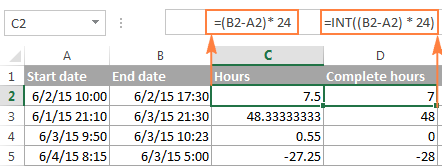
Supposing that your start time is in A2 and end time in B2, you can use a simple equation B2-A2 to calculate the difference between two times, and then multiply it by 24, which is the number of hours in one day:
=(B2-A2) * 24
To get the number of complete hours, use the INT function to round the result down to the nearest integer:
=INT((B2-A2) * 24)
Total minutes between two times:
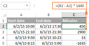
To calculate the minutes between two times, multiply the time difference by 1440, which is the number of minutes in one day (24 hours * 60 minutes = 1440).
As demonstrated in the following screenshot, the formula can return both positive and negative values, the latter occur when the end time is less than the start time, like in row 5:
=(B2-A2)*1440
Total seconds between times:
To get the total seconds between two times, you multiply the time difference by 86400, which is the number of seconds in one day (24 hours * 60 minutes * 60 seconds = 86400).
In our example, the formula is as follows:
=(B2-A2)* 86400
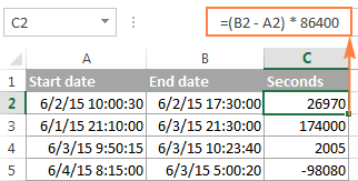
Note. For the results to display correctly, the General format should be applied to the cells with your time difference formula.
Formula 4. Calculate difference in one time unit ignoring others
To find the difference between 2 times in a certain time unit, ignoring the others, use one of the following functions.
- Difference in hours, ignoring minutes and seconds:
=HOUR(B2-A2) - Difference in minutes, ignoring hours and seconds:
=MINUTE(B2-A2) - Difference in seconds, ignoring hours and minutes:
=SECOND(B2-A2)
When using Excel's HOUR, MINUTE and SECOND functions, please remember that the result cannot exceed 24 for hours and 60 for minutes and seconds.

Note. If the end time is less than the start time (i.e. the result of the formula is a negative number), the #NUM! error is returned.
Formula 5. Calculate elapsed time from a start time to now
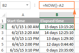
In order to calculate how much time has elapsed since the start time to now, you simply use the NOW function to return today's date and the current time, and then subtract the start date and time from it.
Supposing that the beginning date and time is in call A2, the formula below returns the following results, provided you've applied an appropriate time format to column B, h:mm in this example:
=NOW()-A2
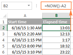
In case the elapsed time exceeds 24 hours, use one of these time formats, for example d "days" h:mm:ss like in the following screenshot:
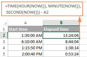
If your starting points contain only time values without dates, you need to use the TIME function to calculate the elapsed time correctly. For example, the following formula returns the time elapsed since the time value in cell A2 up to now:
=TIME(HOUR(NOW()), MINUTE(NOW()), SECOND(NOW())) - A2
Note. The elapsed time is not updated in real-time, it refreshes only when the workbook is reopened or recalculated. To force the formula to update, press either Shift + F9 to recalculate the active spreadsheet or hit F9 to recalculate all open workbooks.
Formula 5. Display time difference as "XX days, XX hours, XX minutes and XX seconds"
This is probably the most user-friendly formula to calculate time difference in Excel. You use the HOUR, MINUTE and SECOND functions to return corresponding time units and the INT function to compute the difference in days. And then, you concatenate all these functions in a single formula along with the text labels:
=INT(B2-A2) & " days, " & HOUR(B2-A2) & " hours, " & MINUTE(B2-A2) & " minutes and " & SECOND(B2-A2) & " seconds"

To instruct your Excel time difference formula to hide zero values, embed four IF functions into it:
=IF(INT(B2-A2)>0, INT(B2-A2) & " days, ","") & IF(HOUR(B2-A2)>0, HOUR(B2-A2) & " hours, ","") & IF(MINUTE(B2-A2)>0, MINUTE(B2-A2) & " minutes and ","") & IF(SECOND(B2-A2)>0, SECOND(B2-A2) & " seconds","")
The syntax may seem excessively complicated, but it works :)

Alternatively, you can calculate time difference by simply subtracting the start time from the end time (e.g. =B2-A2), and then apply the following time format to the cell:
d "days," h "hours," m "minutes and" s "seconds"
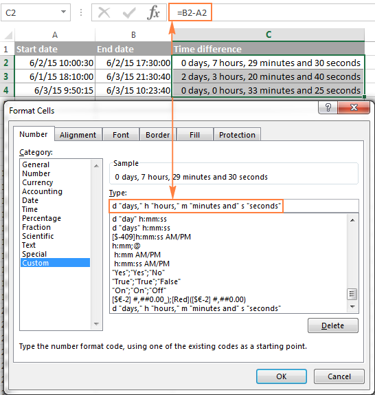
An advantage of this approach is that your result would be a normal time value that you could use in other time calculations, while the result of the complex formula discussed above is a text value. A drawback is that the custom time format cannot distinguish between zero and non-zero values and ignore the latter. To display the result in other formats, please see How to show time over 24 hours, 60 minutes, 60 seconds.
How to calculate and display negative times in Excel
When calculating the time difference in Excel, you may sometimes get the result as ###### error because the difference is a negative time. But is there a way to show negative times properly in Excel? Of course, there is a way, and even more than one :)
Method 1. Change Excel Date System to 1904 date system
The fastest and easiest way to display negative time normally (with a minus sign) is switching to the 1904 date system. To do this, click File > Options > Advanced, scroll down to the When calculating this workbook section and put a tick in the Use 1904 date system box.
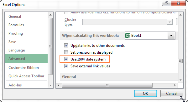
Click OK to save the new settings, and from now on negative times will be displayed correctly, like negative numbers:

Method 2. Calculate negative time in Excel with formulas
Is changing Excel's default Date System is not an option, then you can force negative times to display properly using one of the following formulas:
=IF(A2-B2>0, A2-B2, "-" & TEXT(ABS(A2-B2),"h:mm"))
=IF(A2-B2>0, A2-B2, TEXT(ABS(A2-B2),"-h:mm"))
Both formulas check if the time difference (A2-B2) is greater than 0, and if it is they return that difference. If the time difference is less than zero, the first formula calculates the absolute difference and concatenates the minus sign. The second formula yields exactly the same result by using a negative time format "-h::mm".

Note. Please keep in mind that unlike the first method that treats negative times as negative numeric values, the result of the TEXT function is always a text string that cannot be used in calculations or other formulas.
Adding and subtracting time in Excel
Basically, there are 2 ways to add and subtract time in Excel:
- Using the TIME function
- Using arithmetic calculations based on the number of hours (24), minutes (1440) and seconds (86400) in one day
The TIME(hour, minute, second) function makes Excel time calculations really easy, however it does not allow adding or subtracting more than 23 hours, or 59 minutes, or 59 seconds. If you are working with bigger time intervals, then use one of the arithmetic calculations demonstrated below.
How to add or subtract hours to time in Excel
To add hours to a given time in Excel, you can use one the following formulas.
TIME function to add under 24 hours
For example, if your start time is in cell A2, and you want to add 2 hours to it, the formula is as follows:
=A2 + TIME(2, 0, 0)
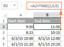
Note. If you try adding more than 23 hours with the TIME function, the specified hours will be divided by 24 and the remainder will be added to the start time value. For example, if you try to add 25 hours to "6/2/2015 10:00 AM" (cell A4) using the formula =A4 + TIME(25, 0, 0), the result will be "06/02/2015 11:00", i.e. A4 + 1 hour.
Formula to add any number of hours (under or over 24 hours)
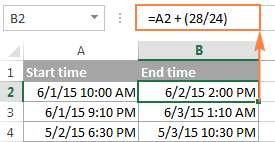
The following formula has no limitations to the number of hours you want to add:
For example, to add 28 hours to the start time in cell A2, enter the following formula:
=A2 + (28/24)
To subtract hours from a given time, you use analogous formulas, and just replace "+" with the minus sign:
For example, to subtract 3 hours from the time in cell A2, either of the following formulas will do:
=A2-(3/24)
=A2-TIME(3,0,0)
To subtract more than 23 hours, use the first one.
How to add / subtract minutes to time in Excel
To add minutes to a given time, employ the same techniques that we've just used for adding hours.
To add or subtract under 60 minutes
Use the TIME function and supply the minutes you want to add or subtract in the second argument:
And here are a couple of real-life formulas to calculate minutes in Excel:
To add 20 minutes to the time in A2: =A2 + TIME(0,20,0)
To subtract 30 minutes from the time in A2: =A2 - TIME(0,30,0)
To add or subtract over 60 minutes
In your calculation, divide the number of minutes by 1440, which is the number of minutes in a day, and add the quotient to the start time:
To subtract minutes from time, simply replace plus with the minus sign. For example:
To add 200 minutes: =A2 + (200/1440)
To subtract 300 minutes: =A2 -(300/1440)

How to add / subtract seconds to a given time
Second calculations in Excel are done in a similar fashion.
To add under 60 seconds to a given time, you can use the TIME function:
To add more than 59 seconds, use the following formula:
To subtract seconds, utilize the same formulas with the minus sign (-) instead of plus (+).
In your Excel worksheets, the formulas may look similar to these:
To add 30 seconds to A2: =A2 + TIME(0,0,31)
To add 1200 seconds to A2: =A2 + (1200/86400)
To subtract 40 seconds from A2: =A2 - TIME(0,0,40)
To subtract 900 seconds from A2: =A2 - (900/86400)
How to sum time in Excel
The Excel sum time formula is the usual SUM function, and applying the proper time format to the result is what does the trick.
Supposing you have a few project times in column B and you want to add them up. You write a simple SUM formula like the one below and get the result in the default format such as hh:mm:ss.
=SUM(B2:B4)
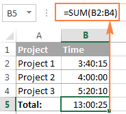
In some cases the default time format works just fine, but sometimes you may want more, for example to display the total time as minutes and seconds, or seconds only. The good news is that no other calculations are required, all you have to do is apply custom time format to the cell with the SUM formula.
Right click the cell and select Format Cells in the context menu, or press Ctrl + 1 to open the Format Cells dialog box. Select Custom from the Category list and type one of the following time formats in the Type box:
- To display total time as minutes and seconds: [m]:ss
- To display total time as seconds: [ss]
The result will look as follows:
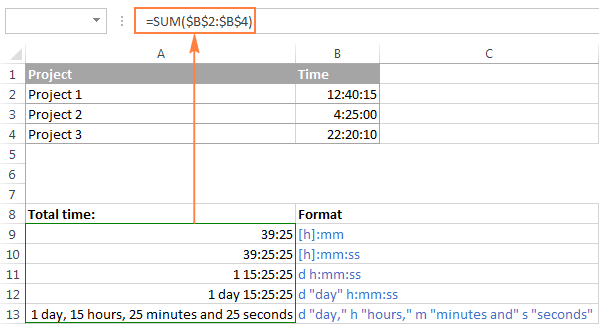
In order to add up more than 24 hours, you use the same SUM formula as discussed above, and apply one of the following time formats to the cell: To see how these custom time formats may look like in your Excel worksheet, please have a look at the screenshot below, where the same SUM formula is entered in cells A9 to A13: Note. The above custom time formats work for positive values only. If the result of your time calculations is a negative number, e.g. when you are subtracting a bigger time from a smaller time, the result will be displayed as #####. To display negative times differently, please see custom format for negative time values.
Also, please keep in mind that the time format applied to a cell changes only the display presentation without changing the cell's value. For example, in the screenshot above, cell A13 looks like text, but in fact it's a usual time value, which is stored as a decimal in the internal Excel system. Meaning, you are free to refer to that cell in other formulas and calculations. For more information, please see How to calculate and show over 24 hours, 60 minutes, 60 seconds.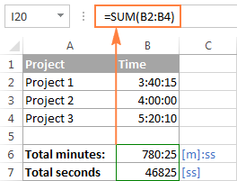
How to sum over 24 hours in Excel
Format
Displays as
Explanation
[h]:mm
30:10
Hours and minutes
[h]:mm:ss
30:10:20
Hours, minutes and seconds
[h] "hours", mm "minutes", ss "seconds"
30 hours, 10 minutes, 20 seconds
d h:mm:ss
1 06:10:20
Days, hours, minutes and seconds
d "day" h:mm:ss
1 day 06:10:20
d "day," h "hours," m "minutes and" s "seconds"
1 day, 6 hours, 10 minutes and 20 seconds
=SUM($B$2:$B$4)
Date & Time Formula Wizard - quick way to calculate times in Excel
Now that you know a bunch of different formulas to add and subtract times in Excel, let me show you the tool that can do it all. Okay, almost all :)
Here comes Ablebit's Date & Time Formula Wizard for Excel:

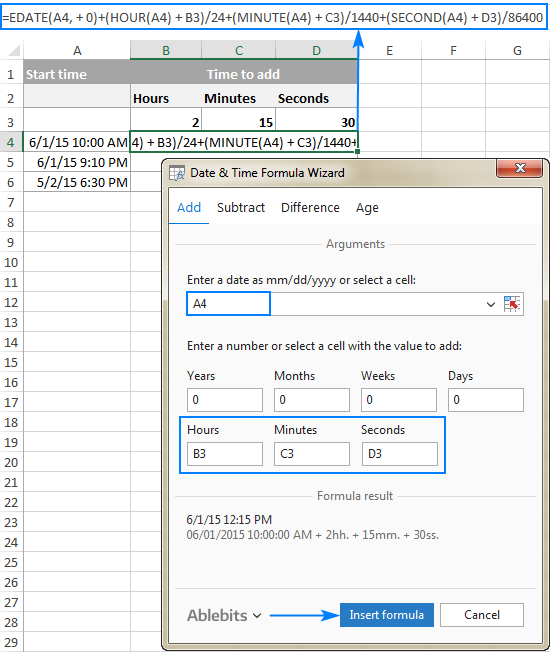
In the Date & Time Wizard dialog window, you switch to the Add or Subtract tab, depending on which operation you want to perform, and do the following:
- Click the Show time fields link in the left part of the window.
- Supply values or cell references for the formula arguments. As you fill in the argument boxes, the wizard builds the formula in the selected cell.
- When finished, click the Insert Formula
That's it! For example, this is how you can add the specified number of hours, minutes and seconds to the time in A4:
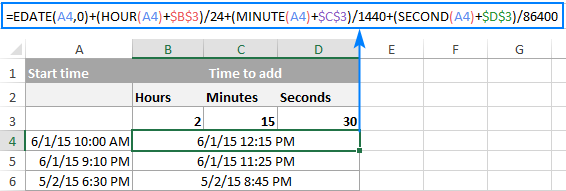
If you need to copy the formula to other cells, fix all references except the cell containing the original time (A4) with the $ sign like shown in the screenshot below (by default, the wizard always uses relative references). Then double-click the fill handle to copy the formula down the column and you are good to go!
Besides time calculations, the wizard can also add and subtract dates, get the difference between two dates, and calculate age from the birthdate.
If you are curious to try this tool in your own worksheets, you are welcome to download the evaluation version of our Ultimate Suite below.
This is how you calculate time in Excel worksheets. To learn other ways to manipulate dates and times in Excel, I encourage you to check out the resources at the end of this article. I thank you for reading and hope to see you on our blog next week!
Available downloads
Excel Time Calculations - formula examples (.xlsx file)
Ultimate Suite - trial version (.exe file)
 by
by
977 comments
Hi !
Anyone help me ! How to find out the Max time while matching two scenarios
I am unable to calculate 24 hours time in excel if anybody knows please help me...
Hi Sunil,
Hopefully you will find an answer here:
How to add & subtract time in Excel to show over 24 hours, 60 minutes, 60 seconds
Hello,
I have a start time and end time for hundreds of people, some people multiple start and end times since they clock in and out multiple times per time. I also have a week's worth of data. How can I extract the total amount of time that falls between two specific times. So I only want to know how many hours, minutes, seconds each person worked between 10AM - 12PM specifically for each day. Also is there a way to customize, make the dates interchangeable, times interchangeable? I may need to look up total hours for multiple days/time periods. My Data looks like this:
Last Name Date St art End Total Hours
Chiang 12/9/18 0.00
Cota 12/9/18 0.00
Cuevas Chairez 12/12/18 11:05:00 AM 6:15:00 PM 7.17
Cuevas Chairez 12/9/18 5:48:00 AM 10:35:00 AM 4.78
Davila 12/9/18 0.00
Flores 12/9/18 10:21:00 AM 5:17:00 PM 6.93
Flores 12/10/18 5:00:00 AM 9:50:00 AM 4.83
Holguin 12/11/18 8:54:00 AM 5:24:00 PM 8.50
THANK YOU for any help you can provide. I have been stumped on this for weeks!!
if i use a single cell to to schedule a shift such as: 8:00AM-4:00PM is there a way to calculate the total hours worked minus a half hour break in the next cell? EG /7.50
Beginning Time = 8:20 PM
Ending time = 4:32 AM
(Over Nite Sleep in hours/minutes)
I'm a beginner. Thanks
Bob
Hello, Bob,
If your cells contain the time values only, please try to use the formula like the one below:
=IF(Ending Time < Beginning Time, Ending Time+1, Ending Time) - Beginning Time
Just change the Beginning and Ending Time to your cell references.
Hope this is what you need.
I plot out the wildlife sightings from my trial cam. Specifically, I obtain the time and date attributes of each .jpg photo and plot them out. But, after daylight savings time I have to subtract one hour from the time. I have that figured out, but when the time and date are 11/11/2018 0:38, for example, subtracting one hour should be 11/10/2018 23:38. But instead I get ########… Also, the correct response needs to be in a plottable format, not text. I'm stumped. Please help.
Hi Dave,
Assuming the original time is in A2, you can use this formula to subtract 1 hour:
=A2-(1/24)
If the formula cell displays ########, just make the column a little wider to accommodate the date/time value.
my formula is giving abrupt values. don't know why?
suppose ...
A1= 08:00 Hrs.
A2= 07:00 Hrs.
A3 =01:00 Hrs.
A4= IF(A1-(A2+A3)<0,"ERR",(A1-(A2+A3)))
with current values of A2 & A3 the result is "ERR" but it should be 0 i think.
Hi,
check in check out
28/10/2018 08:03 28/10/2018 19:57
29/10/2018 19:58 30/10/2018 07:54
30/10/2018 19:55 31/10/2018 07:56
I'm looking for a formula that calculate how many hours i have been in between 19;00 and 22:00.
Thanks
I am looking for a formula that will populate fields for me automatically to count down seconds. Starting at 10:00, counting down to 9:00. 10:00...9:59...9:58 and so on.
Thanks
Hi,
I am using these formulas to calculate slary cost. I have now been ble to make A2 the start of the shift, B2 the end of the shift, C2 the duration of the shift. How can I make D2 = Total salary cost for the shift (based of C2)
Thanks
Hi,
I have the time sheet, In that i have to segregate the 1-5 min, 5-10 min, 10-15 min ect.. to calculate the no of 1-5 min and 5-10 min and 10-15 min. Kindly help me.
Caption under figure in Formula 4 should say "less than" it seems.
Hi Dave,
Absolutely so. Fixed, thank you!
Is there a way to calculate time with a format where you just use 7-4. Meaning that the 7 would in the AM and the 4 bing in the PM
Outstanding explanations!! This (=IF(INT(B2-A2)>0…) was exactly what I needed. That you for the excellent explanations and demos.
Hi All,
I'd really appreciate some help with this. I'm trying to calculate a time cost per spend for a restaurant split between Pre 17:00 & post 17:00.
I have in column A start time and column B finishing time.
So it could be: 09:00 18:59 or 19:03 01:15 or 09:30 16:11
How can I calculate the hours pre 17:00 without it adding straight up to 17:00 and calculate the the ones post 17:00 without it adding in extra time or going negative due to going past the midnight threshold.
I'd really appreciate an answer because it is racking my brains something rotten.
Kind regards
Nick
I have successfully used formula:
=IF(INT(W47-V47)>0,INT(W47-V47)&" days, ","")&IF(HOUR(W47-V47)>0,HOUR(W47-V47)&" hours, ","")&IF(MINUTE(W47-V47)>0,MINUTE(W47-V47)&" minutes")
but am getting FALSE for some Minutes and #NUM when time is set to same day.
Any ideas?
How fields Look
Previous Current Time between Events
End Event
Time Start
3/13/18 16:48 4/20/18 05:31 37 days, 12 hours, 43 minutes
4/20/18 05:31 4/24/18 18:43 4 days, 13 hours, 12 minutes
4/24/18 18:43 6/16/18 00:00 52 days, 5 hours, 17 minutes
6/16/18 00:00 6/21/18 00:43 5 days, 43 minutes
6/21/18 00:43 7/02/18 06:43 11 days, 6 hours, FALSE
7/02/18 06:43 7/10/18 06:14 7 days, 23 hours, 31 minutes
7/10/18 06:14 7/10/18 19:55 13 hours, 41 minutes
7/10/18 19:55 7/31/18 06:00 20 days, 10 hours, 5 minutes
7/31/18 06:00 8/03/18 08:47 3 days, 2 hours, 47 minutes
8/03/18 08:47 8/08/18 03:36 4 days, 18 hours, 49 minutes
8/08/18 03:36 8/10/18 10:48 2 days, 7 hours, 12 minutes
8/10/18 10:48 8/14/18 04:48 3 days, 18 hours, FALSE
8/14/18 04:48 8/14/18 01:12 #NUM!
8/14/18 01:12 8/17/18 17:31 3 days, 16 hours, 19 minutes
8/17/18 17:31 8/30/18 09:11 12 days, 15 hours, 40 minutes
V column is calculated as =TEXT(A60,"m/dd/yy ")&TEXT(R60,"HH:MM")
W column is calculated as =TEXT(A61,"m/dd/yy ")&TEXT(R61,"HH:MM")
where
A60 is a manually entered field say 8/30/2018
and
A61 is a manually entered field say 8/17/2018
and
R60 and R61 is a manual entered field for outage time Say 5.5 representing 5 hours and 30 minutes.
Thanks
Cell A1 is having 20-09-2018 18:14:10
Cell B1 is having 20-09-2018 20:00:30
Objective is to find the time difference and used B1-A1.
But error is coming like this #VALUE!
Appreciate if you can suggest solution to get the time difference.
Siva:
I believe this is a formatting issue. Your Excel doesn't recognize 20-09-2018 as a date.
So, then the idea is to get the date formatted in a way your Excel sees as a date. The way it stands, Excel sees it as text.
Try changing the two dates to 9/20/2018, leave the time as is and see if you can then simply subtract the cells using B1-A1. If that works then you need to work on the formatting issue.
Try changing the formatting of the cells to the date using the location option. In the Date there's the option to specify a locale or location. Find yours and change it there.
You can try replacing the "-" with "/" and see if that works.
If these approaches don't work, then you can split the dates and times into two columns, then split the dates into three columns and concatenate them into one cell using DATEVALUE, format the cell as Date subtract the cells and Bob's your uncle. This sounds harder than it is, in fact I used this last approach many times with data sets containing thousands of rows of data.
Let me know how it goes.
Cell A1 is having 20-09-2018 18:14:10
Cell B1 is having 20-09-2018 20:00:30
Objective is to find the time difference and used B1-A1
As per your suggestion, I changed the date part to 09/20/2018 and applied B1-A1, it worked. But it is difficult to change it manually in all cells. Tried to format the cell using the location option. It didn't work if I replace the "-" with "/". Please suggest workable solution. My file is having thousands of rows of data with this format.
I have a start_date and end_date, wants to calculate the number of hours & minutes between the date excluding weekends as well as time from 12:00 AM to 8:00 AM.
Start_date End_Date Hour spend (excluding weekends & time between 12AM to 8AM)
6/5/2018 6:54:15 PM 6/10/2018 11:28:46 PM
Your prompt response is highly appreciated.
Thanks & Regards
Chander
Hello !
I´m struggeling with making a calculation between two times that consists of minute, seconds, hundredths
ex 01:54,36
The calculation should be
00:47,26 - 00:46,58 = DIFF
or
01:14,29 -01:16,32 = DIFF
or
01:13,12 - 00:56,24 = DIFF
The examples shows that the first time could be either faster och slower then the second one.
Any ideas ?
Thank you.
1935 to 0135 how many hours
time in time out total hrs
6:29:41 AM 5:28:07 PM ?
6:44:17 AM 4:57:45 PM ?
this is the case
- our time in should be 7am and hrs should be counted from 7am to 11:30 for the morning time and from 1:30 pm onwards whatever the time is.
- i want to know the formula for this.
- lunch break should be less from 11:30am to 1:00pm same with 6:00pm to 7:00pm
Anurika:
I think this is what you're looking for.
Where the time data is in E1 enter this in an empty cell:
=IF(E1<=TIME(9,0,0),E1,"0:00")
Now, you can format the cells as Time and you can work with the data as time.
Hi,
Please help me.
ColumnA ColumnB
4:00 4:00
5:00 5:00
11:00 00:00
10:00 00:00
3:00 3:00
This is my question.
I need to get the hours which are below 9:00 to columnB from ColumnA as i showed above.Please give a formula.
Thank you.
we will calculate the time as indian time how to calculate
Start time 07:00 AM
End time 02:00 AM
I have a question. I work in payroll at my work and we have 2 shifts. Is there an easy way to calculate differential time. What I mean is like this
We have shifts that start at 14:20 and the differential kicks in at 18:00 and they work to 22:50. Is there a way for excel to calculate the amount of differential time that they worked?
It would be nice if there was a way to do total time and differential time but since the guys cant make up their mind when they want to go to lunch it makes flat calculations hard. It is always nice to have the computer back up your numbers too.
Adam:
Do the employees clock in and out during their shifts?
Are these times recorded in Excel?
What's the differential pay?
Hai good day
Dear plz tell me how Sum in excel sheet day,hour,and minutes
Exampla: "4 days 3 hours 45 minute and 16 second"
Riaz:
What other times do you want to sum?
Hi,
I need a solution for excel sheet I am maintaining to track activities on issues I get from client.
Working hours are 09.00 am to 05.00 pm and every issue has 4 hours of time to get it acknowledged for the first time. For every issue creating after 05.00 pm (today) till 09.00 am(next day) must calculate acknowledge time from 09.00 am.
How can we do this?
Thank you,
Ankita
Hi,
I am calculating retirement remaining years, while i used "Yearfrac" formula, all went good. but still some is not functioning, ex. one person already reached to retire in the previous year and formula is not showing -1 year, its showing remaining 1. please someone help me to get out from this problem.
Thank you,
Safiur Rahman
How can I get an AVERAGE of start times, Cleaning crew starts cleaning equipment at different times due to production:
Mon cleaning crew started at 12:50AM (entered as 00:50)
Tue cleaning crew started at 12:15AM (entered as 00:15)
Wed cleaning crew started at 12:10AM (entered as 00:10)
Thu cleaning crew started at 23:45PM (entered as 23:45)
Fri cleaning crew started at 23:50AM (entered as 23:50)
I need an AVAERAGE start time for the week.
Using AVERAGE(D4:D8) gives me 09:46AM. I'm looking for a time closer to 00:16. I appreciate your help, thank you in advance.
Greg
Greg:
Try entering the time as 12:50, 12:15, etc. and then AVERAGE. When I do this the return is 12:10.
If I
have
Specific hour (3:30am) and I want to use in a formula to calculate how many employee punched after 3:30 am
I will appreciate your help.
Thanks for your time and help
I just want to add durations (D5 through D308)...I need a total in hrs, mins, and seconds. DOes anyone know a formula for this?
Joe:
If the data in D5:D308 is formatted as Custom [h}:mm:ss
you should be able to sum them with SUM(D5:D308) or whatever combination of cells you need to sum.
Right click, Format Cells, Custom and choose the [h]:mm:ss option.
Thanks Doug, I've been doing exactly as you prescribed and I'm only getting 0:00:00. I'll gladly try anything else you might have. Thanks
My data has a start time and end time for a behaviour
i.e.
09:20:45 09:21:09 So this behaviour lasted for 24 seconds
09:21:09 09:21:30 So this behaviour lasted for 21 seconds
I have 20,000 data points. I am looking for a formula to look for all behaviours that occur only on the minute. So in the example above, only the first data point would be marked true as the second point does not occur on the minute. In this example, the first data point would be the data point for 09:21:00 and the second data point would be deleted.
I hope that makes sense!
Desperately need formula for the following:
If < 6.05, then subtract .50
Thanks
Darren:
Where the data is in cell A1 the formula is:
=IF(A1<6.05,(A1-0.5),"Number is Bigger than 6.05")
If your data is in another cell, enter that cell address in place of A1.
After you've entered the formula in the appropriate cell, you can copy it down the column to calculate more cells.
2-May-18 4:35 1-May-18 14:19 HOW CAN I CALCULATE DIFF IN HOUR
Manoj:
The formula is:
=((End Date + End Time)-(Start Date + Start Time))*24
i want to know how to calculate time when u have a negative sign. see example below:
if
start time end time Hours worked
7:45am 3:15pm ???
so what is the way forward?
Hello, Andrew:
There are three ways negative time can be displayed in Excel. The first two ways are explained in the article above this post, so no need to rehash them here. I would recommend you use one of them.
The third way is to custom format the cell holding the negative time as -h:mm. This method works only if you always want a negative time value displayed. It also requires that you always subtract the earlier time from the later time. This means times returned really will be positive and will only appear negative. Probably not the best method.
I am hosting a running event where people guess how fast they can run a mile, then they run the mile, and I have to be able to calculate the difference between their guess and what they actually ran, but I can't figure out how to format the cells because everything is in time as it relates to the day. I type in 5.22 to represent 5 minutes and 22 seconds but no matter what I put as the format it changes it to 5:22 am or pm and throws off the calculation. Can someone please help???
Tiffany:
If you change the format of the cells that will contain the times to h:mm the cells and the subsequent calculations will work the way you want.
Select the cells, then right click and choose Format Cells, then choose Custom where you will find the h:mm option in the list. I know it means "hours:minutes" but maybe for your purposes it will work.
Hi there,
I am trying to calculate the time difference of the following function on my excel spreadsheet;
=TEXT(E4-D4,"HH:MM:SS") and i press enter but it gives me #VALUE
what does that mean and if you can help solve this...it took me an hour to fix this
thanks
bobby
Bobby
Bobby
What do you have in E4 and D4? Are the values in there formatted as time?
Hi there,
I am trying to calculate the time difference of the following function on my excel spreadsheet;
=TEXT(E4-D4,"HH:MM:SS") and i press enter but it gives me #VALUE
what does that mean and if you can help solve this...it took me an hour to fix this
thanks
Bobby
Hello, please help me with the formula for below:
Example 1:
If email Time received Date & Time =25/5/2018 18:00 Hrs and email processed Date and Time is 26/5/2018 14:15 Hrs
Example 2:
If email Time received Date & Time =25/5/2018 22:01 Hrs and email processed Date and Time is 26/5/2018 14:15 Hrs
The time should calculate total hours taken only between my shift is 13:00 to 22:00 Hrs. If email received is after 22:00 hrs the total time taken to process should calculate from next day 13:00Hrs
Hi Doug, any thoughts here?
Ramana:
After much searching I found a solution that works for your situation and several others, too.
The solution is waaaay too complicated to type here, so I'll provide the link.
You'll want to download the sample workbook that is at the bottom of the article as it is really nice and contains all the examples and formulas on several sheets.
To download the workbook click the enlarge icon at the bottom right of the embedded worksheet. When you can see the big sheet, click on the download button at the top of the sheet.
The link to the site is: https://www.exceltactics.com/calculate-net-work-hours-using-networkdays/
Suppose opening quantity of JW Black Lable whisky (750 ml)1.300ml ie,1 bottle & 300 ml.received from godown is 1(750ml) bottle, so total is 2.3 ie,2 bottle & 300 ml.And sale is .6 ml ie,600 ml.what formula to be used to get the closing stock in one cell.
Hello! Is there a predefined formula for calculating time it takes to complete a project if the data are in seconds or min/unit?
Example: 1 unit = 15sec, 5 units must be completed
Therefore, 5 units = 1 min:15 sec
10 units = 2 min:15 sec
Trying to estimate packaging times for product units. Thanks!
Ash:
Not sure of your question, but try this and see if it works for you:
Enter this in say B2 =IF(A10<1,0,A10)
Where A10 is the cell that holds the data.
You can format B2 to show the number of decimal places to fit your needs.
please help me...
i need formula that if the excess hour is less than 1hr it will answer to 0:00 and if its 1hr to up it will show the excess hour starting only in 1hr to up.
is it possible??/
thank you
sign in time sign out time Late Attendence Work Hours
10:12:07 17:21:11 0:12:07 7:09:04
Start Time 10:00:00 AM
End Time = 17:00:00 PM
That's amazing formula which is this
=IF(INT(B2-A2)>0, INT(B2-A2) & " days, ","") & IF(HOUR(B2-A2)>0, HOUR(B2-A2) & " hours, ","") & IF(MINUTE(B2-A2)>0, MINUTE(B2-A2) & " minutes and ","") & IF(SECOND(B2-A2)>0, SECOND(B2-A2) & " seconds","")
But i have problem if the second is 0 the result is like this
"33 minutes and"
How to get rid " and" in this case?
I'm using the following formula to calculate the number of working hours.
The result is a decimal number which can be later multiplied by the hourly rate if you need to.
For ex.
8h 15min = 8.25hrs
You can also enter the time over the midnight.
Ex.
Start 20:00 Finish 04:00 = 8.00h
=IF(E10=0,0,IF(E10>D10,(E10-D10)*24,(24-D10*24+E10*24)))
D10 - Start time
E10 - Finish time
Time format 12:00:00
Hi Yuriy Roshchupkin,
can you give me the formula for to change 8h 15min to 8.25hrs.
Thanks
Aditya
thanks a lot.
this one im looking for 1hour
Hi Yuriy Roshchupkin,
I tried your formula with the exact data that you have and it gave me a zero as the answer. The Time format is the same, is there something that I am missing?
please tell me how to do this calculation in excel.
calculation should done by right side to left side
(signs-degrees-minutes-seconds)
(12-30-60-60)
Example for Addition:-
09-20-13-40
00-13-10-35
------------
10-03-24-15
------------
Example for Subtraction:-(in the below case we cannot delete 8 from 7. because we get 1 minute from minutes (i.e. 60 seconds) and from 67 seconds subtract 08 seconds)
03-10-05-07
00-00-04-08
-----------
03-10-00-59
-----------
i need code for this calcultion.
Thanks
Sankar.
How I protect the cell from adding or deleting at a certain time. for example:
I do not add or delete on this cell from 1:00 PM to 2:00 PM at 04/20/2018.
Is there a formula in Excel? Please
Hi
Good Day
Please help me in excel sheet
Start Time Finish Time Mints
07:00am 17:00pm ?
Note: we don't want create any new calm & line between Start Time and Finish Time.
Change 17:00pm to 05:00pm and it should work. 1700 is 24 hour format while 05:00pm is 12 hour format. You cannot calculate using two different time formats.
use this formula to calculate diffidence between both of time .mod(finish time-start time,1)
Please data to data calculate send mi