In this article I'll show you 3 ways how you can add hyperlinks into your Excel workbook to easily navigate between numerous worksheets. You'll also learn how to change a link destination and modify its format. If you don't need a hyperlink any more, you'll see how to quickly remove it.
If you are a real Internet surfer, you know firsthand about the bright sides of hyperlinks. Clicking on hyperlinks you instantly get access to other information no matter where it is located. But do you know the benefits of spreadsheet hyperlinks in Excel workbooks? The time has come to discover them and start using this great Excel feature.
One of the ways you can put spreadsheet hyperlinks to good use is to create a table of contents of your workbook. Excel internal hyperlinks will help you to quickly jump to the necessary part of the workbook without hunting through multiple worksheets.
Insert a hyperlink in Excel
If you need to add a hyperlink in Excel 2016 or 2013, you can choose one of the following hyperlink types: a link to an existing or new file, to a web page or e-mail address. Since the subject of this article is creating a hyperlink to another worksheet in the same workbook, below you'll find out three ways to do that.
Add a hyperlink from the context menu
The first method of creating a hyperlink within one workbook is to use the Hyperlink command.
- Select a cell where you want to insert a hyperlink.
- Right-click on the cell and choose the Hyperlink option from the context menu.
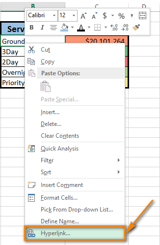
The Insert Hyperlink dialog window appears on the screen. - Choose Place in This Document in the Link to section if your task is to link the cell to a specific location in the same workbook.
- Select the worksheet that you want to link to in the Or select a place in this document field.
- Enter the cell address in the Type the cell reference box if you want to link to a certain cell of another worksheet.
- Enter a value or name into the Text to display box to represent the hyperlink in the cell.
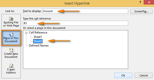
- Click OK.
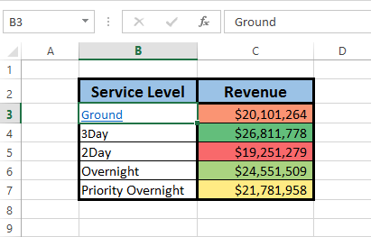
The cell content becomes underlined and highlighted in blue. It means that the cell contains the hyperlink. To check if the link works, just hover the pointer over the underlined text and click on it to go to the specified location.
Excel HYPERLINK function
Excel has a HYPERLINK function that you can also use for creating links between spreadsheets in the workbook. If you are not good at entering Excel formulas immediately in the Formula bar, do the following:
- Select the cell to which you want to add a hyperlink.
- Go to Function Library on the FORMULAS tab.
- Open the Lookup & Reference drop-down list and choose HYPERLINK.
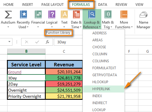
Now you can see the function name in the Formula bar. Just enter the following two HYPERLINK function arguments in the dialog window: link_location and friendly_name.
In our case link_location refers to a specific cell in another Excel worksheet and friendly_name is the jump text to display in the cell.
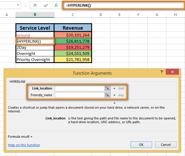
Note. It's not a must to enter friendly_name. But if you want the hyperlink to look neat and clear, I'd recommend to do it. If you don't type in friendly_name, the cell will display the link_location as the jump text.
- Fill in the Link_location text box.

Tip. If you don't know what address to enter, just use the Select range icon to pick the destination cell.
The address displays in the Link_location text box.

- Add the number sign (#) before the specified location.
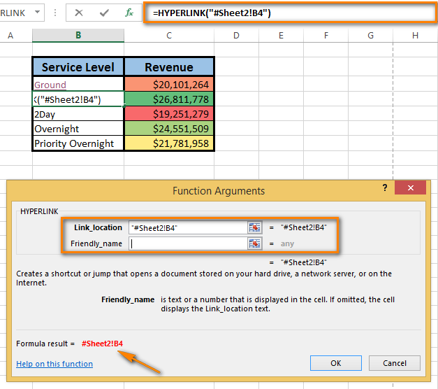
Note. It is crucial to type the number sign. It indicates that the location is within the current workbook. If you forget to enter it, the link won't work and an error will appear when you click on it.
When you move to the Friendly_name text box, you see the formula result in the bottom-left corner of the Function Arguments dialog.
- Enter Friendly_name that you want to display in the cell.
- Click OK.
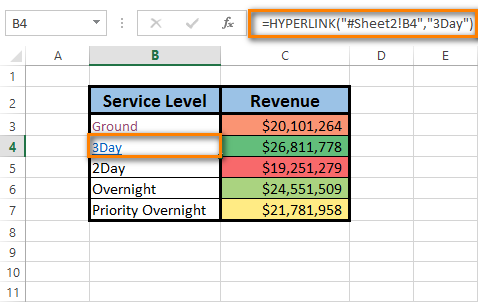
Here you are! Everything is as it should be: the formula is in the Formula bar, the link is in the cell. Click on the link to check where it follows.
Insert a link by cell drag-and-drop
The quickest way of creating hyperlinks within one workbook is using the drag-and-drop technique. Let me show you how it works.
As an example, I'll take a workbook of two sheets and create a hyperlink in Sheet 1 to a cell in Sheet 2.
Note. Make sure that the workbook is saved because this method doesn't work in new workbooks.
- Select the hyperlink destination cell in Sheet 2.
- Point to one of the cell borders and right-click.
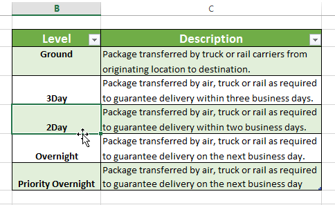
- Hold the button and go down to the sheet tabs.
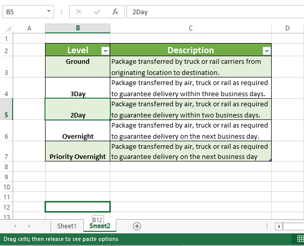
- Press the Alt key and mouse over the Sheet 1 tab.
Having the Alt key pressed automatically takes you to the other sheet. Once Sheet 1 is activated, you can stop holding the key. - Keep dragging to the place where you want to insert a hyperlink.
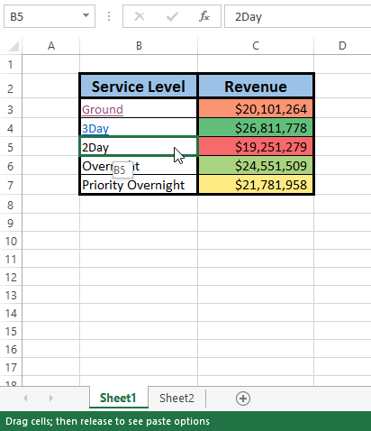
- Release the right mouse button for the popup menu to appear.
- Choose Create Hyperlink Here from the menu.
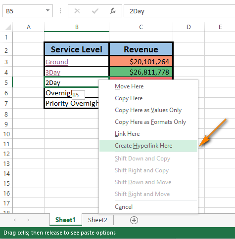
After you do that, the hyperlink appears in the cell. When you click on it, you'll switch to the destination cell in Sheet 2.
No doubt that dragging is the fastest way to insert a hyperlink into an Excel worksheet. It combines several operations into a single action. It takes you less time, but a bit more attention concentration than two other methods. So it's up to you which way
to go.
Edit a hyperlink
You can edit an existing hyperlink in your workbook by changing its destination, its appearance, or the text that is used to represent it.
Change link destination
As this article deals with hyperlinks between spreadsheets of the same workbook, the hyperlink destination in this case is a specific cell from another spreadsheet. If you want to change the hyperlink destination, you need to modify the cell reference or choose another sheet. You can do both, if necessary.
- Right-click the hyperlink you want to edit.
- Choose Edit Hyperlink from the popup menu.
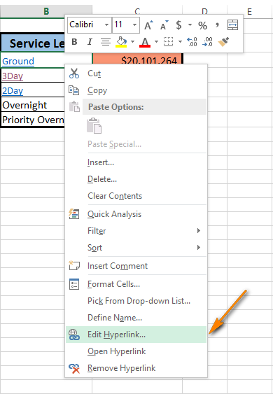
The Edit Hyperlink dialog box appears on the screen. You see that it looks the same as the Insert Hyperlink dialog and has the identical fields and layout.
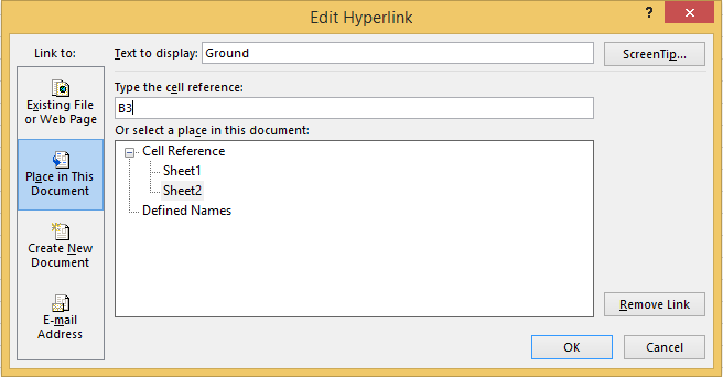
Note. There are, at least, two more ways to open the Edit Hyperlink dialog. You can press Ctrl + K or click on Hyperlink in the Links group on the INSERT tab. But don't forget to select the necessary cell before doing it.
- Update the information in the appropriate fields of the Edit Hyperlink dialog.
- Click OK and check where the hyperlink jumps to now.
Note. In case you used Method 2 to add a hyperlink in Excel, you need to edit the formula to change the hyperlink destination. Select the cell that contains the link, and then place the cursor in the Formula bar to edit it.
Modify hyperlink format
Most of the time hyperlinks are shown as an underlined text of blue color. If the typical appearance of hyperlink text seems to you boring and you'd like to stand out of the crowd, go ahead and read below how to do it:
- Go to the Styles group on the HOME tab.
- Open the Cell Styles list.
- Right-click on Hyperlink to change the appearance of the hyperlink that was not clicked. Or right-click Followed Hyperlink if the hyperlink was activated.
- Choose the Modify option from the context menu.
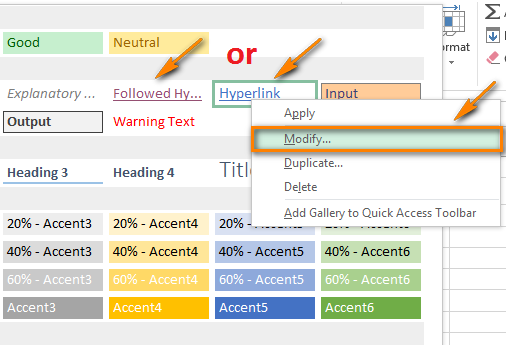
- Click on Formatin the Styles dialog box.
- Make the necessary changes in the Format Cells dialog window. Here you can change the hyperlink alignment and font or add fill color.
- When you are done, click OK.
- Make sure that all the changes are marked under Style includes in the Style dialog box.
- Press OK.
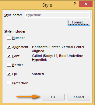
Now you can enjoy a new individual style of the hyperlinks in your workbook. Pay attention that the changes you made affect all the hyperlinks in the current workbook. You can't change the appearance of a single hyperlink.
Remove a hyperlink
It will take you a few seconds and no efforts to delete a hyperlink from the worksheet.
- Right-click the hyperlink you want to remove.
- Choose the Remove Hyperlink option from the popup menu.
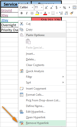
The text remains in the cell, but it is no longer a hyperlink.
Note. If you want to delete a hyperlink and the text that represents it, right-click the cell that contains the link and choose the Clear Contents option from the menu.
This trick helps you to delete a single hyperlink. If you want to know how to remove multiple (all) hyperlinks from Excel worksheets at a time, follow the link to our previous blog post.
I hope that in this article you saw the simplicity and effectiveness of using internal hyperlinks in a workbook. Just a few clicks to create, jump and discover the massive content of complex Excel documents.
 by
by
127 comments
Good write up.
Very very helpful.
Can we hyperlink between the two cells of different sheet of same excel file matching the text of cell?
Thank you. I got many benefit from here.
None of this is working for me. Directions don't match what I'm seeing and pictures don't show the #, so where does it go? I used to do this stuff in Excel all the time, but now that I have Windows 10 and office 16, it seems like everything is so difficult. Every time I look for instructions, the instruction pictures don't match what I'm seeing on screen.
Thanks!!!
Hyperlink it make the task simple
Thank you
Hi,
how to hyperlink with formula if the sheet names are in number?
Thanks.
Kinsen
Quite useful.Thank you.
Thank you so much, it was clearly explained and easy to follow. Will be back again I'm sure.
hey
Thanks For information but i want to link cell to worksheet of wps spreadsheet
please let me know the information..
thanks and regards
Mauryaa Bhalerao
Late to the party.
"Insert a link by cell drag-and-drop"
This works, but is there a way to create the link automatically? If a cell in sheet four matches a cell in sheet one, can the Sheet 4 cell have a hyperlink to the Sheet 1 cell automatically?
I can flag the duplicates with conditional formatting, but I just can't figure out the next step. Possibly a "IF/THEN statement?
Its very precise and composed article. much appreciated !!
The info about including the "#" was excellent and saved heaps of time and frustration.
Very helpful simple excel tips and hacks. Thank you so much!
Hello,
I like your blog Insert a hyperlink in Excel and really nice information about hyperlink types. Thanks for this information.
I am Planning to put a print button in excel file.
Scenario is:
I am having one Excel file in that one Master Sheet and other 4 sheets are There.
In Master Sheet I want four print buttons for these 4 other sheets.
So that Print button Assigned for Sheet 1 in Master Sheet will print that Sheet 1 from Master sheet itself no need of going to sheet 1.
Same for other sheets.
Truly fantastic. Thanks a million
Thank you so much. I have no enough proficient in Excel Usage. Thank you for your helpful.
thankyou
Seriously your site is helpful and very revealing.
Thanks
Hi I am trying to link a specific name on one tab and once i click on it find that specific name on the next tab is this possible?
Great...Thank a lot.
100% working and helpful
i wanted to insert a hyperlink to a worksheet displaying the worksheet name dynamically, so if i rename the worksheet, the hyperlink display changes to the new name. is there a solution?
"Insert a link by cell drag-and-drop"
It WORKS!!!!
Thank you SO much. Hours of work saved.
Thank you you make it nice and easy to follow and very explicit diagrams!
THANK YOU
Respected Sir,
In our factory there is 3 types of product.
So I will maintain the records in daily basis on EXCEL sheet.(Sheet1)
Sheet 1: There is A type of product are manufacture on 16/09/2016 will be 2 Qty, after that 20/09/2016 will be 3 Qty.Total Qty of A= ,2+3=5
How to link Total Qty of A in Sheet1 to the Total Qty of Sheet2
Sheet1.
SR.NO DATE PRODUCT QTY
1 16/09/16 A 2
2 17/09/17 B 2
3 18/09/18 C 3
4 19/09/19 C 6
5 20/09/20 A 3
Sheet2.
SR.NO PRODUCT TOTAL QTY
1 A
2 B
3 C
How to link Sheet 1 of product to the sheet 2
Just i will enter the Qty in Sheet1 (on Daily basis ), Automatically total Qty of products coming towords sheet2.
Pls send me solution…
Thank you so much! This information saved my bacon!
Please say me solution
It's Awesome one !! Thanks
It seems pretty useless if the link has to go the file location even when linking to a different sheet in the same workbook. If that is the case, the links won't work if you send the file to someone who can't access your file location (ie.. external client). There should be a way to simply have the workbook refer directly to other cells or sheets in the same workbook without need to access the location where the file is stored on your computer. Am I missing something?
Does this hyperlink works only with the Sheet1 only or can we rename the sheet name ??
From a dropdown list of set values, (Yes and No) I am trying to link Yes to another tab
When I hyperlink it, Yes and No both take you to the linked tab
Nice.
Can you hyperlink from one cell in one document to another cell in a separate document? Basically, I want to be able to click on a cell and it open the other document at the same place.
Nothing I have tried has worked.
Excellent! I have, quite literally, found the missing link.
It was all in the need for the #, which I've not seen documented before. Great job, thanks.
how to connection data to another excel sheets
for example
1.book1
2.book2
now i have 10 data in book1 but now while i changed 15 data in book1.
but it automatic changed in book2.
excellent posting. very useful
very very effective info thanks.
Very useful info. Thank You
I have never seen the tip to add the "#" before the target of the link to indicate that the link is in the current worksheet. It works exactly as I would want it to and is impervious to file name or location changes. In contrast, adding a link using the insert hyperlink dialogue (even when speciying that it is within the current workbook) results in a file name being inserted into the link which falls apart if either the filename, or its location, is changed.
Thank you very much!!!
I have been trying to hyperlink between two sheets in the same workbook, and your "Insert a link by cell drag-and-drop" method is the ONLY one that hasn't resulted in an "cannot open the specified file" error message. THANK YOU :)
When I use the first method to create HYPERLINK to another sheet, it says "cannot open the file specified".
Little help here.. :)
Justin, make sure you put in the # before the sheet name. I suspect your error is related to this omission on your formula.
SUPER!!!!!!!!!!!
Hello, is there a way for the selected cell to go to the top of the page? Currently the hyperlink goes to a cell like A124 and that is displayed at the bottom of the page. How can I create a hyperlink that will go to that page and display A124 at the top of the page? Any assistance would be greatly appreciated!
Yes, tell it to go to A1, insetad of A124. Right click, edit and the second box is the cell that you want it to reference.
Is there a way to connect a filter with the link? For example: I have a table of monthly sales. My hyperlink is the sales quantity for each month. My data that is feeding my table (where the hyperlink is connected) has all of my sales quantity by month. I would like to be able to click the hyperlink and have my source filter down based on the month. Is this possible with the hyperlink function?
HI i want to to find out the Cell references in the next sheet, Example in sheet1 i have data 1 to 10 and in Sheet2 the has the data 1 to 10. i need to know the matching cell referneces. in sheet 2 if 1 is at D9, the formulae should show the cell references D9. Is there any formulae like that.
but what if I insert a row before the destination cell? will the hyperlink self adjust to continue pointing to the originally intended destination cell, or would I need to manually adjust the hyperlink to point to the new destination?
Please, someone, answer Chris' enquiry, as I need to know the answer too. And if possible a method of auto-updating the link, if possible. (in Excel 2019)
Hello!
Unfortunately, the hyperlink formula cannot keep track of any changes that occur on the target sheet.
Very useful. Thank You.
good thank u