The article provides detailed guidance on how to use conditional formatting Icon Sets in Excel. It will teach you how to create a custom icon set that overcomes many limitations of the inbuilt options and apply icons based on another cell value.
A while ago, we started to explorer various features and capabilities of Conditional Formatting in Excel. If you haven't got a chance to read that introductory article, you may want to do this now. If you already know the basics, let's move on and see what options you have with regard to Excel's icon sets and how you can leverage them in your projects.
Excel icon sets
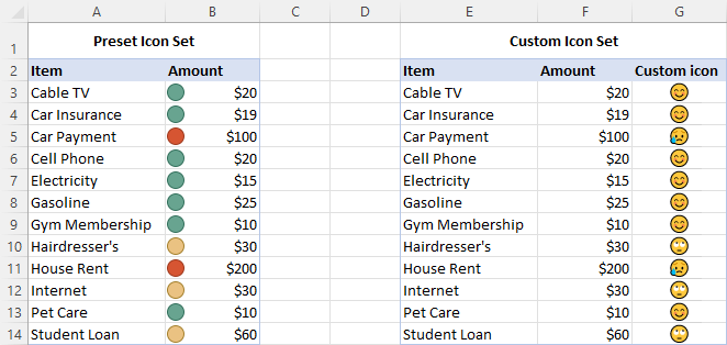
Icon Sets in Excel are ready-to-use formatting options that add various icons to cells, such as arrows, shapes, check marks, flags, rating starts, etc. to visually show how cell values in a range are compared to each other.
Normally, an icon set contains from three to five icons, consequently the cell values in a formatted range are divided into three to five groups from high to low. For instance, a 3-icon set uses one icon for values greater than or equal to 67%, another icon for values between 67% and 33%, and yet another icon for values lower than 33%. However, you are free to change this default behavior and define your own criteria.
How to use icon sets in Excel
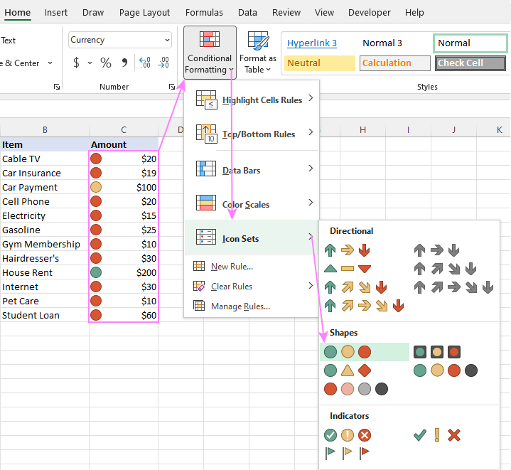
To apply an icon set to your data, this is what you need to do:
- Select the range of cells you want to format.
- On the Home tab, in the Styles group, click Conditional Formatting.
- Point to Icon Sets, and then click the icon type you want.
That's it! The icons will appear inside the selected cells straight away.
How to customize Excel icon sets
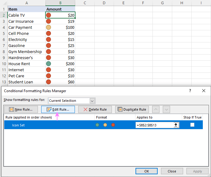
If you are not happy with the way Excel has interpreted and highlighted your data, you can easily customize the applied icon set. To make edits, follow these steps:
- Select any cell conditionally formatted with the icon set.
- On the Home tab, click Conditional Formatting > Manage Rules.
- Select the rule of interest and click Edit Rule.
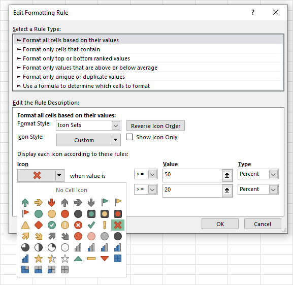
- In the Edit Formatting Rule dialog box, you can choose other icons and assign them to different values. To select another icon, click on the drop-down button and you will see a list of all icons available for conditional formatting.
- When done editing, click OK twice to save the changes and return to Excel.
For our example, we've chosen the red cross to highlight values greater than or equal to 50% and the green tick mark to highlight values less than 20%. For in-between values, the yellow exclamation mark will be used.
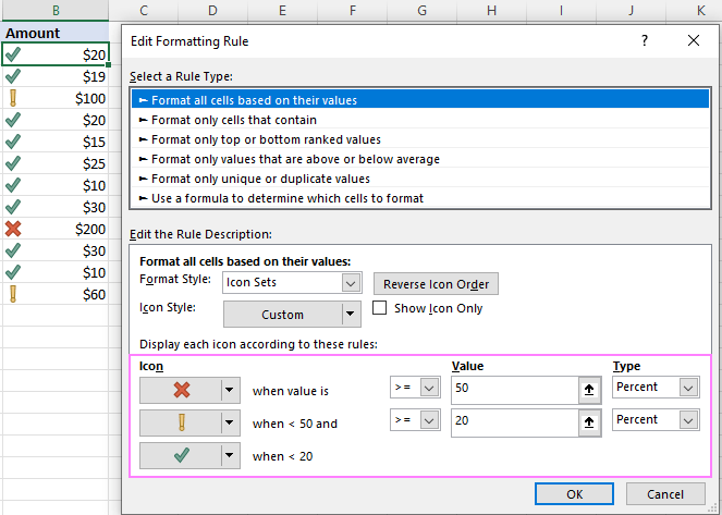
Tips:
- To reverse icon setting, click the Reverse Icon Order button.
- To hide cell values and show only icons, select the Show Icon Only check box.
- To define the criteria based on another cell value, enter the cell's address in the Value box.
- You can use icon sets together with other conditional formats, e.g. to change the background color of the cells containing icons.
How to create a custom icon set in Excel
In Microsoft Excel, there are 4 different kinds of icon sets: directional, shapes, indicators and ratings. When creating your own rule, you can use any icon from any set and assign any value to it.
To create your own custom icon set, follow these steps:
- Select the range of cells where you want to apply the icons.
- Click Conditional Formatting > Icon Sets > More Rules.
- In the New Formatting Rule dialog box, select the desired icons. From the Type dropdown box, select Percentage, Number of Formula, and type the corresponding values in the Value boxes.
- Finally, click OK.
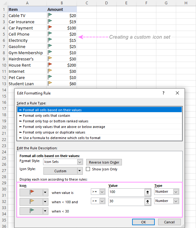
For this example, we've created a custom three-flags icon set, where:
- Green flag marks household spendings greater than or equal to $100.
- Yellow flag is assigned to numbers less than $100 and greater than or equal to $30.
- Green flag is used for values less than $30.
How to set conditions based on another cell value
Instead of "hardcoding" the criteria in a rule, you can input each condition in a separate cell, and then refer to those cells. The key benefit of this approach is that you can easily modify the conditions by changing the values in the referenced cells without editing the rule.
For example, we've entered the two main conditions in cells G2 and G3 and configured the rule in this way:
- For Type, pick Formula.
- For the Value box, enter the cell address preceded with the equality sign. To get it done automatically by Excel, just place the cursor in the box and click the cell on the sheet.
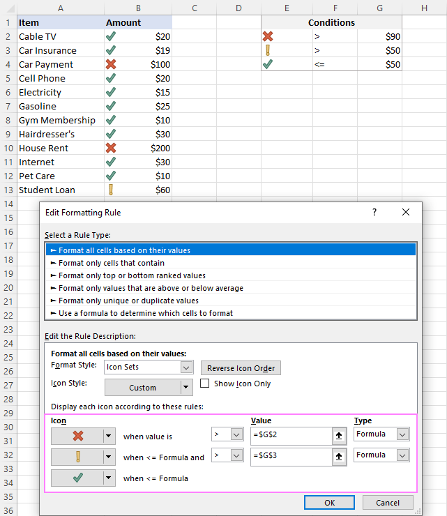
Excel conditional formatting icon sets formula
To have the conditions calculated automatically by Excel, you can express them using a formula.
To apply conditional formatting with formula-driven icons, start creating a custom icon set as described above. In the New Formatting Rule dialog box, from the Type dropdown box, select Formula, and insert your formula in the Value box.
For this example, the following formulas are used:
- Green flag is assigned to numbers greater than or equal to an average + 10:
=AVERAGE($B$2:$B$13)+10 - Yellow flag is assigned to numbers less than an average + 10 and greater than or equal to an average - 20.
=AVERAGE($B$2:$B$13)-20 - Green flag is used for values lower than an average - 20.
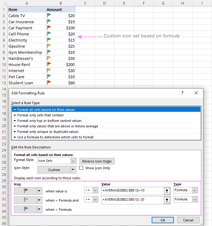
Note. It's not possible to use relative references in icon set formulas.
Excel conditional format icon set to compare 2 columns
When comparing two columns, conditional formatting icon sets, such as colored arrows, can give you an excellent visual representation of the comparison. This can be done by using an icon set in combination with a formula that calculates the difference between the values in two columns - the percent change formula works nicely for this purpose.
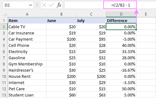
Suppose you have the June and July spendings in columns B and C, respectively. To calculate how much the amount has changed between the two months, the formula in D2 copied down is:
=C2/B2 - 1
Now, we want to display:
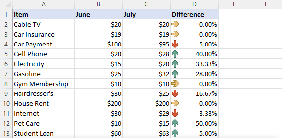
- An up arrow if the percent change is a positive number (value in column C is greater than in column B).
- A down arrow if the difference is a negative number (value in column C is less than in column B).
- A horizontal arrow if the percent change is zero (columns B and C are equal).
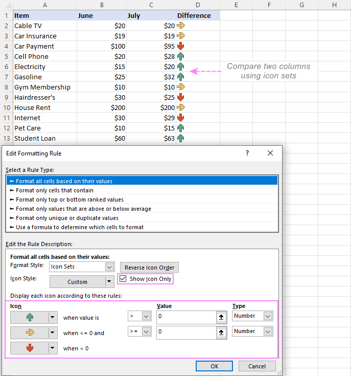
To accomplish this, you create a custom icon set rule with these settings:
- A green up arrow when Value is > 0.
- A yellow right arrow when Value is <=0 and >=0, which limits the choice to zeros.
- A red down arrow when Value is < 0.
- For all the icons, Type is set to Number.
At this point, the result will look something like this:
To show only the icons without percentages, tick the Show Icon Only checkbox.
How to apply Excel icon sets based on another cell
A common opinion is that Excel conditional formatting icon sets can only be used to format cells based on their own values. Technically, that is true. However, you can emulate the conditional format icon set based on a value in another cell.
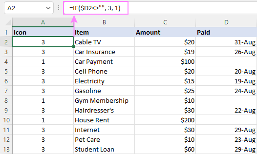
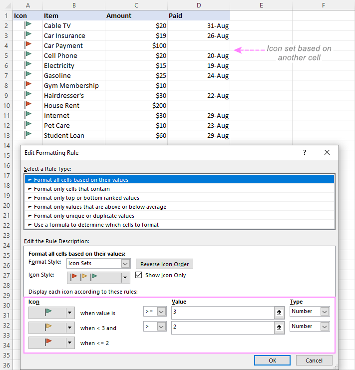
Suppose you have payment dates in column D. Your goal is to place a green flag in column A when a certain bill is paid, i.e. there is a date in the corresponding cell in column D. If a cell in column D is blank, a red flag should be inserted.
To accomplish the task, these are the steps to perform:
- Start with adding the below formula to A2, and then copy it down the column:
=IF($D2<>"", 3, 1)The formula says to return 3 if D2 is not empty, otherwise 1.
- Select the data cells in column A without the column header (A2:A13) and create a custom icon set rule.
- Configure the following settings:
- Green flag when the number is >=3.
- Yellow flag when the number is >2. As you remember, we do not really want a yellow flag anywhere, so we set a condition that will never be satisfied, i.e. a value less than 3 and greater than 2.
- In the Type dropdown box, pick Number for both icons.
- Select the Icon Set Only checkbox to hide the numbers and only show the icons.
The result is exactly as we were looking for: the green flag if a cell in column D contains anything in it and the red flag if the cell is empty.
Excel conditional formatting icon sets based on text
By default, Excel icon sets are designed for formatting numbers, not text. But with just a little creativity, you can assign different icons to specific text values, so you can see at a glance what text is in this or that cell.
Suppose you've added the Note column to your household spendings table and want to apply certain icons based on the text labels in that column. The task requires some preparatory work such as:
- Make a summary table (F2:G4) numbering each note. The idea is to use a positive, negative, and zero number here.
- Add one more column to the original table named Icon (it's where the icons are going to be placed).
- Populated the new column with a VLOOKUP formula that looks up the notes and returns matching numbers from the summary table:
=VLOOKUP(C2, $F$2:$G$4, 2, FALSE)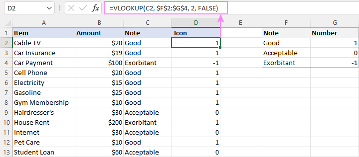
Now, it's time to add icons to our text notes:
- Select the range D2:D13 and click Conditional Formatting> Icon Sets > More Rules.
- Choose the icon style you want and configure the rule as in the image below:
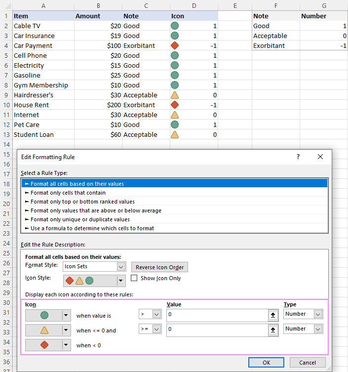
- The next step is to replace the numbers with text notes. This can be done by applying a custom number format. So, select the range D2:D13 again and press the CTRL + 1 shortcut.
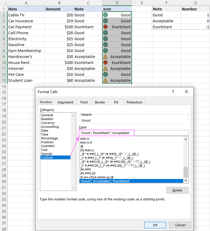
- In the Format Cells dialog box, on the Number tab, select the Custom category, enter the following format in the Type box, and click OK:
"Good";Exorbitant";"Acceptable"
Where "Good" is the display value for positive numbers, "Exorbitant" for negative numbers, and "Acceptable" for 0. Please be sure to correctly replace those values with your text.
This is very close to the desired result, isn't it?
- To get rid of the Note column, which has become redundant, copy the contents of the Icon column, and then use the Paste Special feature to paste as values in the same place. However, please keep in mind that this will make your icons static, so they won't respond to changes in the original data. If you are working with an updatable dataset, skip this step.
- Now, you can safely hide or delete (if you replaced the formulas with calculated values) the Note column without affecting the text labels and symbols in the Icon column. Done!
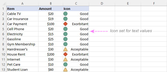
Note. In this example, we've used a 3-icon set. Applying 5-icon sets based on text is also possible but requires more manipulations.
How to show only some items of the icon set
Excel's inbuilt 3-icon and 5-icon sets look nice, but sometimes you may find them a bit inundated with graphics. The solution is to keep only those icons that draw attention to the most important items, say, best performing or worst performing.
For example, when highlighting the spendings with different icons, you may want to show only those that mark the amounts higher than average. Let's see how you can do this:
- Create a new conditional formatting rule by clicking Conditional formatting > New Rule > Format only cells that contain. Choose to format cells with values less than average, which is returned by the below formula. Click OK without setting any format.
=AVERAGE($B$2:$B$13)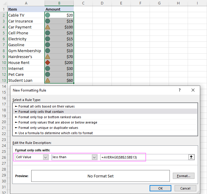
- Click Conditional Formatting > Manage Rules…, move up the Less than average rule, and put a tick into the Stop if True check box next to it.
As a result, the icons are only shown for the amounts that are greater than average in the applied range:
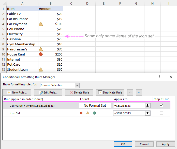
How to add custom icon set to Excel
Excel's built-in sets have a limited collection of icons and, unfortunately, there is no way to add custom icons to the collection. Luckily, there is a workaround that allows you to mimic conditional formatting with custom icons.
Method 1. Add custom icons using Symbol menu
To emulate Excel conditional formatting with a custom icon set, these are the steps to follow:
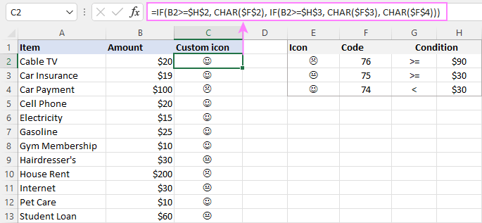
- Create a reference table outlining your conditions as shown in the screenshot below.
- In the reference table, insert the desired icons. For this, clicking the Insert tab > Symbols group > Symbol button. In the Symbol dialog box, select the Windings font, pick the symbol you want, and click Insert.
- Next to each icon, type its character code, which is displayed near the bottom of the Symbol dialog box.
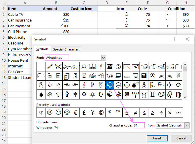
- For the column where the icons should appear, set the Wingdings font, and then enter the nested IF formula like this one:
=IF(B2>=90, CHAR(76), IF(B2>=30, CHAR(75), CHAR(74)))With cell references, it takes this shape:
=IF(B2>=$H$2, CHAR($F$2), IF(B2>=$H$3, CHAR($F$3), CHAR($F$4)))Copy the formula down the column, and you will get this result:
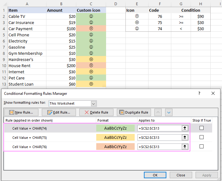
Black and white icons appear rather dull, but you can give them a better look by coloring the cells. For this, you can apply the inbuilt rule (Conditional Formatting > Highlight Cells Rules > Equal To) based on the CHAR formula such as:
=CHAR(76)
Now, our custom icon formatting looks nicer, right?
Method 2. Add custom icons using virtual keyboard
Adding custom icons with the help of the virtual keyboard is even easier. The steps are:
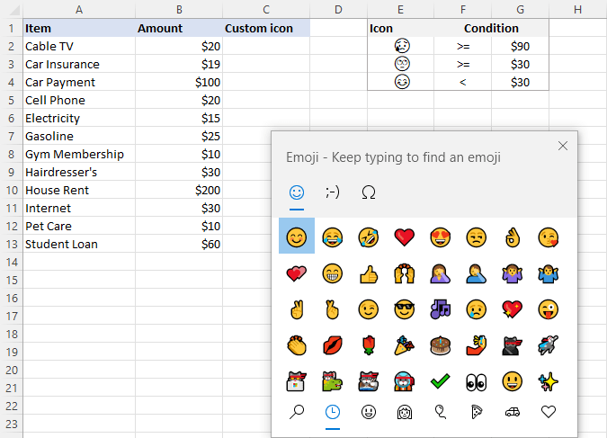
- Start by opening the virtual keyboard on the task bar. If the keyboard icon is not there, right-click on the bar, and then click Show Touch Keyboard Button.
- In your summary table, select the cell where you want to insert the icon, and then click on the icon you like.
Alternatively, you can open the emoji keyboard by pressing the Win + . shortcut (the Windows logo key and the period key together) and select the icons there.
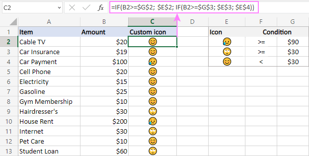
- In the Custom Icon column, enter this formula:
=IF(B2>=$G$2, $E$2, IF(B2>=$G$3, $E$3, $E$4))In this case, you need neither the character codes nor fiddling with the font type.
When added to Excel desktop, the icons are black and white:
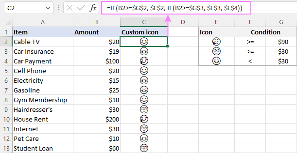
In Excel Online, colored icons look a lot more beautiful:
This is how to use icon sets in Excel. Upon a closer look, they are capable of a lot more than just a few preset formats, right? If you are curious to learn other conditional formatting types, the tutorials linked below may come in handy.
Practice workbook for download
Conditional formatting icon sets in Excel - examples (.xlsx file)
 by
by
162 comments
Hello Svetlana,
I want to change the color of the icon set versus default
I have task list different target based on the load and case type, How can I use the formula?
I want to use the icon sets in reverse order like green color down arrow, red color up arrow to project lower the better values. Is it possible?
hi, i need to use Data Icons in Conditional Format.
if Delivery Date is Greater than or equal today , it should be GREEEN
if Delivery Date is less than today with one week , it should be YELLOW
if Delivery Date is less than 7 Days and lesser , it should be RED
pls send
Hi,
Need support in fetching a particular date from a set number of days of the month (30,31,28)
please see if the formula for the same is pre-fed or has to be calibrated by combining formulae.
Thanks
Dear Svetlana,
I am trying to make a "% completed" column using progress bar that is dependent on "Status", which are of texts instead of numbers. My question here is, is it possible to create progress bar with "Status" e.g. "Stage 1" displaying 10% on the progress bar?
I have tried to use IF formula to relate the "% completed" column to "Status" column, i.e.; =IF($C$6, 0, IF($C$7, 10, IF($C$8, 15, IF($C$9, 20, IF($C$10, 40, IF($C$11, 50, IF($C$12, 60, IF($C$13, 65, IF($C$14, 70, IF($C$15, 80, IF($C$16, 90, IF($C$17, 95, IF($C$18, 100))))))))))))). However, the result is #VALUE!
Dear Good morning,
One question... it's possible to display in a gantt chart a mailstone with flag that use color variable green red or yellow flag in function of status value ?
Many thanks in advanced
Paolo
I want know can conditional format a data for 4 employees in 4 different rows for 3 months in 3 different columns. If they are doing 2 3 4 hours work for 1st employee 4 3 2 for 2nd employee & 3 4 6 hours for 3rd employee & 7 8 9 hours for 4th employee
Now I want to continual format with icon set plz help
hello every one
I would like to use two columns.first one will have temperature data, second one will have symbols like (Suspect or good).Every cells at second column will check the data which at tle left cells at the left column and if there are persist data more than determined number( l will chose it like if there are 10 same temperature data next to next) than will write SUSPECT at the righ column cell .
thank you
Hi,
Please help me to make the icon sets for below calculation.
>85% (Green Color)
>61% to 84% (Yellow)
<61 % (Red)
How can I make?
Thanks
Hi
I am not an advanced Excel user but I wondered if you could help. I have a budget sheet that runs on month after month and I use filters to see what I'm spending in the current month (by filtering out all the previous months). I also assign a different category as I enter each invidual expenditure (food, petrol etc). I also have the monthly budget total for each catagory on a separate sheet.
What I would like to do is see easily, at a glance, when I have spent each budget - whether this is using icons or simply having a list of categories that decrease in value as I spend. I can do this manually by using filters and cross checking on the separate budget sheet but is there a way to do this automatically using forumulas?
Can i change icon colour?
hello friends,
is it possible to put formula depending on icon color,
suppose i already have green, yellow & red in row & i want one cell which represent if all green then green or any one yellow then yellow or any red then red
I wonder if i could do thing like : if cell A equal to cell B format cell C with a symbol tick, if the two cell are not equal format with a symbol X and if i have nothing in cell A or cell B format with symbol!. any help ?
Hi Need help with the below.
I have created a conditional format for one of the cell where the cell, if the cell value is great than the value from the last week show Up arrow, if the same cell value is lower than the value of the previous week show Red down arrow. I am not able to copy this conditional format to the other cell as conditional format marks the initial cell value as $ so when I copy the format it still looks up the first cell from the previous week. Please help.
Hi Svetlana
I have a row of data containing formula that returns a number. I have applied the icon sets to return an icon based on <33rd,67th percentile but when I manually check the sets based on the colours that should be showing they are wrong. Is there anything obvious i should check for? I have copied and pasted values but still get the same result.
Thank you!
Hi Svetlana,
I could really use your assistance. Is it possible to apply an Excel icon set based on the sum/difference of another cells formula =IMSUB(E2,F2)? this is for a running inventory sheet. E2 would be starting stock, F2 would be number of stock used, G2 then shows current stock. I want cell G2 to show icons according to the result of =IMSUB(E2,F2) Thank you for any help.
Hi there, the circular icon sets in excel is limited to three; red, green and yellow. I want to indicate the status of my Action Log as:
-In progress
-Overdue
-Completed
-Postponed
-Cancelled
More than three colours (actually 5) here, any advise on how we can get around to get 5 different coloured circular icons??
Appreciate you advise
John
Sorry * Yellow when >=D2*0.8
I have posted only a part of data I have a load of such target V/s actual figures which are to be indicated with icons. Please suggest any formula in condition formatting icon sets so that I can drag or format paint without the error of relative references
Thanks in advance
D E F G
2 Budgeted 80 90 100 100
3 Actual 80 89 97 97
Icons required in actual (Row 3)
Green-when value >= D2
Yellow-when =D2*0.8
Red-when<formula
But this only works for cell D3, and not for E3, F3 or G3. Need it for a dashboard urgent help please
Update to problem above
Hi,
I want to use icon set formatting in the below scenario:
D6 - revenue 100
D7 - revenue 90
D8 - revenue 95
I want to show icon set in D6 and D7 comparing to D8. so for example D7 is less than D8 so Green up arrow, if it was greater than D8 red arrow down but D6 is greater than D8 so red down arrow and if it was less than D8 then green arrow up.
Any help would be hugely appreciated.
Hi,
I want to use icon set formatting in the below scenario:
D6 - revenue 100
D7 - revenue 90
D8 - revenue 95
I want to show icon set in D6 and D7 comparing to D8. so for example D7 is less than D8 so Green up arrow but D6 is greater than D8 so red down arrow.
Any help would be hugely appreciated.
Hi
I am trying to create a spreadsheet which column A is (Issue Date)Column B (Purposed Date) and Column C (Competition Date ) there are column D (Status)
I want column D highlight (Red, Amber, Green) based on Purposed date if the issue date past purposed date highlight red on column D, and if competition date is before purposed date highlight Green on column D or else Highlight amber if Issue date is not exceed purposed date.
Hope these make sense
Hoping for your views and reply on this
Many Thanks
Emmanuel
Hi,
Suppose i have created a table where i will update my data daily or weekly wise.
Now i want to create another chart or table which just shows a particular color corresponding my values in the table i created but not the value itself.
Is there any formula for that in excel.
Dear Team,
please I would need your expertise touch here.
I have three cells (say A1, B1 and C1) .
A1 is titled "%completed"; B1 "%Tartget" and C1 "Rating/Status"
I would like to be able to compute (use nested if to determined the status of the two cells if the difference btn cell A1 and B1 meets a condition.
***This explains how the ratings are computed.
--Not Started , if value equals zero (0) (black Arrow down)
--Achieved, if %completed is greater than 90 (green Flagged)
--Partly Achieved , if %Comp greater than 50 but less than 90 (Yellow Flagged)
--Not Achieved , if %comp not equal to zero but less or equal to 50 (Red Flagged)
the above is working fine for me but there are instances where cell B1 (%target has a mark of say 48 which will not be achieved according the above creteria.
Please who can achieve this ?
worried,
Fred
i am using the icon set red, yellow and green circles. is it possible to change the color of the icons, they are a bit pale according to my boss. i am in excel 2010
Hi. I'm using Excel 2016. For the Icon Sets, mine are rust, gold and
muted green, not a normal red, yellow, and green as I see in the screenshots above. I tried changing the Theme, but no change. What can I change to get the more traditional colors for the traffic lights?
hi
i have a table consist of 3 columns filled with numbers. i want 3 icons which tell me which data value is maximum, which one is minimum and which is between them?
Hello, I have an excel pivot table that has pulled in data from a sharepoint dashboard file. The cell content indicates RAG of Green, Yellow, Red. Is there a way to apply conditional formatting to interpret those rags and provide icons?
can you help in conditional formatting. I want to know how to fill a cell like vertical bar bottom to above
Hi
Please help me.. i try to make custom icon in conditional formatting, but it cant be save..after reopen the file, the conditional formatting formula not shown..
Need to put stocks but i need put it in one cell i have one target like ...
Target : 90%
The cell : 95.3%
Then i need put stock next to 95.3% in the same cell
Thanks...
Hi - conditional formatting was working well on the data I pulled in to my sheet via a CSV URL feed. The publisher of the feed changed the CSV format (putting the header rows on the bottom--causing me to have to reverse the rows in order to use the first row as the column headers--no big deal there); however, now the conditional formatting no longer works. All the data / columns still the same but it's as if Excel no longer recognizes the type of data in the column--raw from the CSV or formatted manually in Excel. Seems it won't recognize the format. Could formatting be an issue why conditional formatting STOPS working?
Also, i have a formula for that particular column and it is formatted to %, the conditional formatting doesn't work. However, if i change the format to number, apply conditional formatting and then convert the column to %, then it works. Why is this happening?? What is the problem with applying conditional formatting in % formatted cells?
Hi,
I'm trying to get icon sets with following conditions-
If values are >75% represent with Upward arrow
If values are between 30% & 75% represent with Straight line
If values are <30% represent with downward arrow
Please help me on this as i am getting a down arrow for 33% as well?
Thanks
I have conditional formatting on column N which fills different colors based on containing word on it. I want same color to fill on the column A:M based on column N color. Tried many ways to get the same color from formatted column but not succeed. Is there any way to get same color from other the cell?
I am using the Data Bar in Conditional Formatting and my data contains percents. I want the length of the bar to be relative to 0% to 100% but the length of the bar is always relative to the highest percentage value in my data. I've tried changing all the minimum and maximum settings but have not found a fix. Is there a way to do this?
Hi. For an Excel/PPT presentation i would need data change visualization. I would like to do it with the help of the Conditional Formatting - Icon Sets. But i would need other Icons then arrows or the given ones in Excel. Is there a known possibility to somehow import other new icons to Excel for this setting? (For Excel 2010 and 2013)
Thanks in advance.
I am trying to create an excel chart has a date column (Column A) and tasked organizations (columns F thru AB). I am trying to format it so that if the date passes, the organizations that are tasked (not all are assigned at any given point) the box will automatically go black/overdue. Until that date, the box should just be yellow or "pending". I am really confused and tried multiple sites. I am using Excel 2013.
I have a spreadsheet and I am trying to automate a row that will show a green arrow up or red arrow down depending on the relationship between the 2 previous columns. So if the # in column A is greater than the # in column B, I want a green arrow in column C. And vice versa. Any help would be appreciated. I have played around with the Rules under Conditional Formatting, but can't seem to find one that fits what I am trying to do. (Excel 2013) Thanks.
I want to set a cell can display the cut-off time itself and use solid fill function to show may time left.
For example, our time start from 8:30 AM and one of our counter's cut-off time is 9:30 AM. I want this cell always display 9:30 and the data bar will become shorter base on time pass.
Thanks Svetlana!
You really saved my day. Great and clear info. Greetings from Bogotá. :)
I want to use a text value to trigger a conditional formatting icon. Text value being red =(red dot), yellow = (yellow dot), green = (green dot). Can this done?
I want to make a checklist, is there a way to put a checkbox before each item and have code that if there is a check mark in the checkbox it highlights whatever the cell (not row) is to the right of the checkbox?
Hello Jamie,
You can do this with the help of VBA in Excel, you can try posting your question on the VBA branches of the following websites: https://www.excelforum.com/ or https://www.mrexcel.com/
Hi,
I'm trying to set the conditions to act or function this way,
If values are >0% represent with Upward arrow
If values are =0% represent with Straight line
If values are <0% represent with down ward arrow
Anyone has an idea about this?
Please help
Thanks
Hello,
You need to create a conditional formatting rule based on cell values, choose "Icon sets" as the format style, pick the necessary set of icons in the "Icon style" drop-down list and enter the following rules:
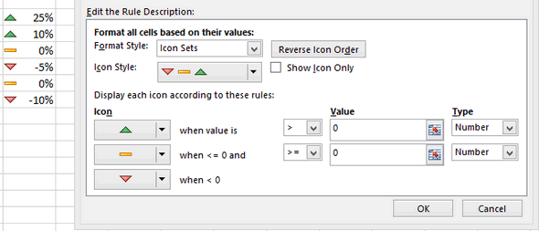
- Show upward arrow when the value is >0 and choose "Number" under "Type"
- Show a straight line when the value is >=0
- The downward arrow will automatically get the condition "when <0":
Hi Svetlana,
I'm that you are helping everyone in the forum with solutions for their question.
I too have a quick question and hope it's easy for you. I would like the values in the column to be represented by icons the condition would be
1. If the values are >10% it must represented by by a upward arrow
2. If the values are >0 %<10% It must be represented by a straight arrow
3. If the values are <0 % It must be represented by a downward arrow.
Hope it's easy for your level of expertise. Many thanks in advance and look
forward to hear from you.
Regards,
Gabriel
Hi Gabriel,
Hopefully, this is what you are looking for:
Hi,need your support on below case, thanks a lot,
I want to the sixth number/color in icon sets, but only five labels in excel sheet,
I have created conditionally formatted icon sets (stoplight) for an array of data. I would like to set up a word mail merge and have the icons (red, yellow, green stoplights) appear in the word doc on mail merge. Instead I seem to only be getting the value of the cell. Any help?